Finite temperature
On this page we compute thermal averages,
There are three methods: purification, METTS and exact diagonalization. METTS is built on imaginary-time evolution, which has its own section.
Purification
Each physical site gets an ancilla site. The product of singlets between each site and its ancilla is a pure state whose reduced density matrix on the physical chain is \(\rho\propto\mathbb 1\), the \(T=\infty\) state. Evolving it in imaginary time with the physical \(H\),
and tracing out the ancillas gives \(\rho(T)\propto e^{-\beta H}\).
from dmrgpy import thermal
n = 6
tc = thermal.Thermal_Spin_Chain(["S=1/2"]*n, T=0.5)
h = sum(tc.Sx[i]*tc.Sx[i+1] + tc.Sy[i]*tc.Sy[i+1] + tc.Sz[i]*tc.Sz[i+1]
        for i in range(n-1))
tc.set_hamiltonian(h)
tc.get_gs()                                   # builds |Psi(beta)>
E = tc.MBChain.vev(h).real                    # thermal energy
czz = tc.MBChain.vev(tc.Sz[0]*tc.Sz[1]).real  # thermal <Sz_0 Sz_1>
tc.Sx, tc.Sy, tc.Sz are the operators of the physical sites, and
tc.MBChain is the doubled chain that holds the purified state. Static
expectation values on tc.MBChain are thermal averages. A dynamical
correlator on tc.MBChain is not the thermal one, so use METTS or ED for
those. T=0 gives the ordinary ground state. The imaginary-time evolution
is accurate to about \(10^{-6}\) relative at the defaults. The keywords are:
tc.anneal_step: the size of each imaginary-time step, in units of the spectral width (default 2). Smaller is more accurate and slower.tc.anneal_order: the order of the expansion of each step (default 8).tc.anneal_method: how \(e^{-\beta H/2}\) is applied."taylor"is the expansion above,"implicit"the implicit steps of Imaginary-time evolution, whose number grows as \(\log\beta\) and not as \(\beta W\), with \(W\) the spectral width. The default,None, takes the implicit steps onitensor_version=3at \(T\le0.05\) (in units of the largest coupling) when they need far fewer solves than the expansion needs steps, that is on long chains, and the expansion otherwise. Settinganneal_steporanneal_orderkeeps the expansion. The implicit steps run onitensor_version=3,"python"and"julia_live".tc.anneal_options: the keywords ofevolve_imaginary_timefor"implicit", exceptshift. The default isorder=8withnsteps=2: the \(T=\infty\) state holds every energy of the spectrum, and the trapezoid rule is not accurate enough for it.tc.MBChain.maxm: the bond dimension of the purified state. It needs to be larger at intermediate temperatures.
See examples/finite_temperature/thermal_purification_VS_exact.
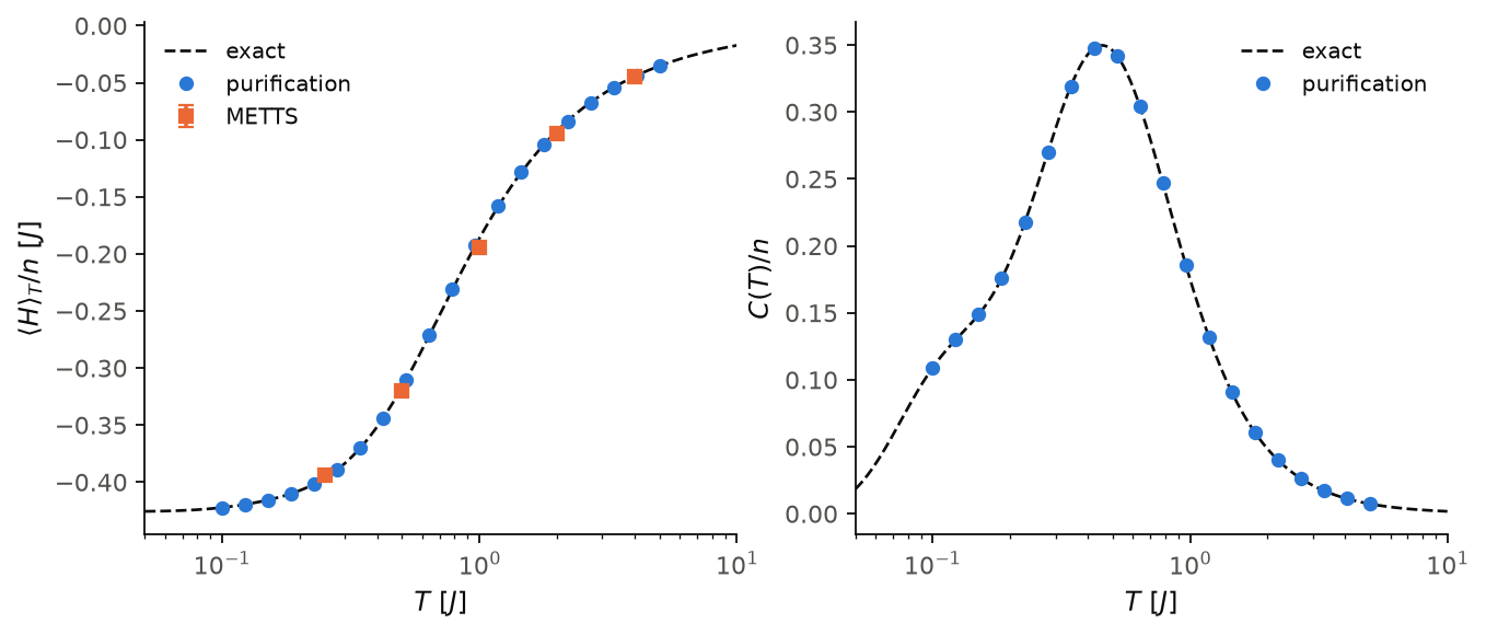
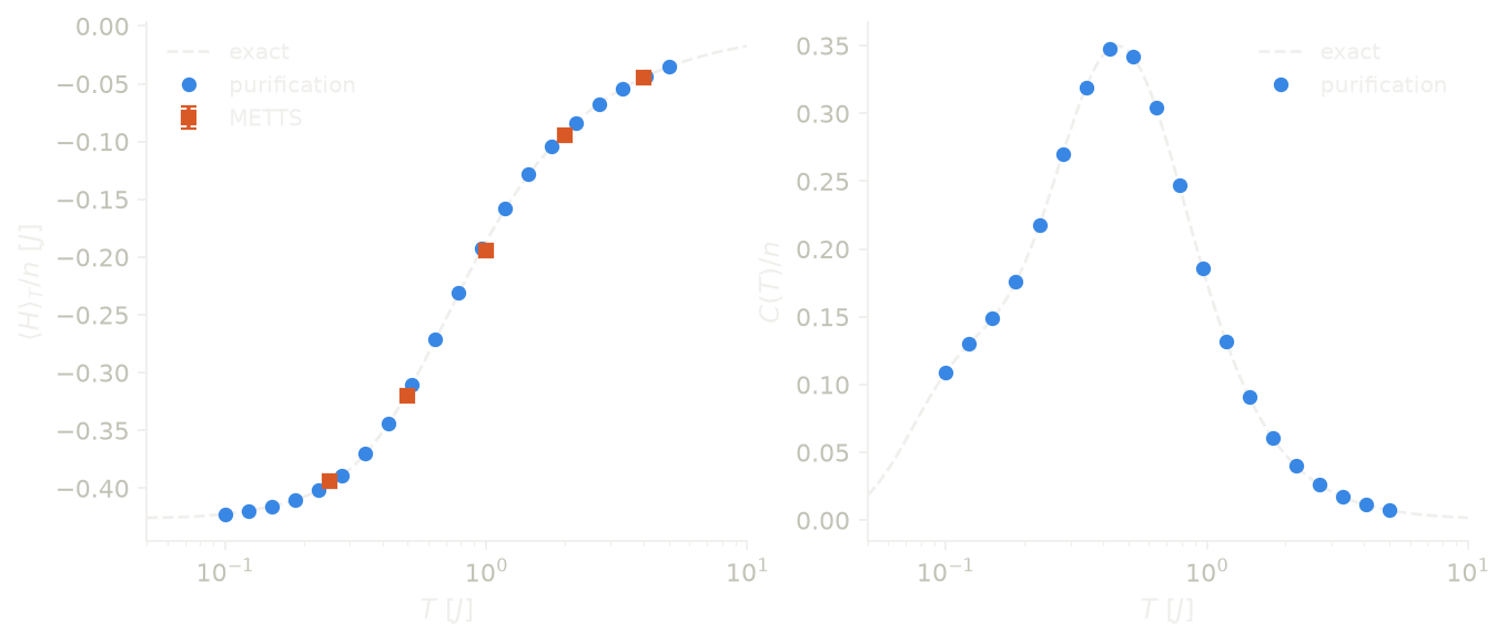
The figure shows the thermal energy and the specific heat per site of a spin-1/2 Heisenberg chain with \(n=10\). The specific heat is the energy variance, \(C(T)=(\langle H^2\rangle_T-\langle H\rangle_T^2)/T^2\), measured in the purified state, so no numerical derivative is needed. The reference is the full spectrum of the chain (dashed lines). Purification agrees with it to \(10^{-5}\) at every temperature. \(C(T)\) has a broad maximum near \(T\approx0.46J\), the scale of the antiferromagnetic correlations. The METTS points are discussed in METTS.
Code of this figure (docs/figures/finite-temperature_specific_heat/)
# Thermal energy and specific heat of the spin-1/2 Heisenberg chain from
# purification and from METTS, against the exact full-spectrum result.
import numpy as np
from dmrgpy import spinchain, thermal

n = 10
T_pur = np.geomspace(0.1, 5, 20)
T_metts = [0.25, 0.5, 1.0, 2.0, 4.0]
T_exact = np.geomspace(0.05, 10, 300)


def heisenberg(c):
    return sum(c.Sx[i]*c.Sx[i+1] + c.Sy[i]*c.Sy[i+1] + c.Sz[i]*c.Sz[i+1]
               for i in range(n-1))


# exact: <H>_T and C = (<H^2>_T - <H>_T^2)/T^2 from all 1024 eigenvalues
sc = spinchain.Spin_Chain(["S=1/2"]*n)
h = heisenberg(sc)
sc.set_hamiltonian(h)
hm = sc.get_ED_obj().get_hamiltonian()
ev = np.linalg.eigvalsh(hm.toarray() if hasattr(hm, "toarray") else hm)
E_exact, C_exact = [], []
for T in T_exact:
    w = np.exp(-(ev - ev.min())/T)
    e, e2 = (ev*w).sum()/w.sum(), (ev**2*w).sum()/w.sum()
    E_exact.append(e)
    C_exact.append((e2 - e**2)/T**2)

# purification, a fresh thermal chain per temperature
E_pur, C_pur = [], []
for T in T_pur:
    tc = thermal.Thermal_Spin_Chain(["S=1/2"]*n, T=T)
    tc.MBChain.maxm = 100
    ht = heisenberg(tc)
    tc.set_hamiltonian(ht)
    tc.get_gs()
    E_pur.append(tc.MBChain.vev(ht).real)
    C_pur.append(tc.MBChain.gs_energy_fluctuation()**2/T**2)

# METTS on the physical chain
E_metts, err_metts = [], []
for T in T_metts:
    e, err = sc.metts_vev(h, T, nsamples=300, nwarmup=30, seed=1)
    E_metts.append(e.real)
    err_metts.append(err)

np.savez("data.npz", n=n, T=T_pur, E_pur=E_pur, C_pur=C_pur,
         T_metts=T_metts, E_metts=E_metts, err_metts=err_metts,
         T_exact=T_exact, E_exact=E_exact, C_exact=C_exact)
import numpy as np
import style

d = np.load("data.npz")
n = d["n"]
T, Te, Tm = d["T"], d["T_exact"], d["T_metts"]


def draw(theme):
    c = style.colors(theme)
    fig, (ax1, ax2) = style.figure(2)
    ax1.plot(Te, d["E_exact"]/n, **style.reference(theme), label="exact")
    ax1.plot(T, d["E_pur"]/n, "o", color=c["series"][0], ms=style.MS,
             label="purification")
    ax1.errorbar(Tm, d["E_metts"]/n, yerr=d["err_metts"]/n, fmt="s",
                 color=c["series"][1], ms=style.MS, capsize=3, label="METTS")
    ax1.set_ylabel(r"$\langle H\rangle_T/n$ [$J$]")
    ax2.plot(Te, d["C_exact"]/n, **style.reference(theme), label="exact")
    ax2.plot(T, d["C_pur"]/n, "o", color=c["series"][0], ms=style.MS,
             label="purification")
    ax2.set_ylabel(r"$C(T)/n$")
    for ax in (ax1, ax2):
        ax.set_xscale("log")
        ax.set_xlabel(r"$T$ [$J$]")
        ax.set_xlim(Te[0], Te[-1])
        ax.legend()
    return fig


style.main(draw, "finite-temperature_specific_heat")
Imaginary-time evolution
Imaginary-time evolution projects a state onto the low energies,
At long \(\tau\) it gives the ground state, and at \(\tau=\beta/2\) it is the step of METTS below. Each eigenstate decays as \(e^{-(E_n-E_0)\tau}\), so the energy scale that matters falls as \(\tau\) grows, and the time steps can grow with it (Zima, Stoudenmire, White, Parcollet and Kaye, arXiv:2606.02930). The grid has panels \([0,\tau_0]\), \([\tau_0,2\tau_0]\), \([2\tau_0,4\tau_0]\), ... up to \(\tau\), with a few equal steps in each, so the number of steps grows as \(\log\tau\) and not as \(\tau\). A long step needs an implicit rule, the trapezoid rule
which is stable for any step size. Each step needs one linear solve. Here
h is the Hamiltonian of the chain and
wf the initial state, for example a Néel state:
wft = sc.evolve_imaginary_time(wf, 100.)     # normalized e^{-100 H}|wf>
taus, e = sc.evolve_imaginary_time_and_measure(h, wf, 100.)
The second call returns the grid times and \(\langle\psi(\tau)|h|\psi(\tau)\rangle\)
on them. With an ED state, mode="ED" gives the exact evolution on the
same grid. In examples/finite_temperature/imaginary_time_log_grid the
Néel state of a 12-site Heisenberg chain reaches \(\tau=1000\) in 72 steps,
and its energy ends \(5\times10^{-12}\) above \(E_0\). The error of the trapezoid
rule falls as \(1/n^2\) with the number \(n\) of steps per panel. It is largest
at intermediate \(\tau\), where the energy is off by about \(2\times10^{-3}\)
(in units of the exchange) at \(n=4\) in that example. The keywords are:
nsteps: the steps per panel (default 4).tau0: the end of the first panel (default 0.01 over the largest coupling of \(H\)). The first steps must resolve the highest energies the initial state contains.order: 2 for the trapezoid rule, 4, 6, ... for the Gauss-Legendre rules, more accurate per step, withorder/2complex linear solves each.shift: the energy subtracted from \(H\), by default the ground-state energy. It must be the ground-state energy: with a lower shift the long steps stop projecting.
It works with itensor_version=3 (at least 3 sites), "python" and
"julia_live", for a Hermitian \(H\).
METTS
Minimally entangled typical thermal states (Stoudenmire and
White, arXiv:1002.1305) sample product states \(|i\rangle\) with a Markov
chain. Each one is evolved to
\(|\phi_i\rangle\propto e^{-\beta H/2}|i\rangle\) and then collapsed to a new
product state. The plain average of \(\langle\phi_i|O|\phi_i\rangle\) over
the chain is the thermal average. The states stay weakly entangled, so
no ancillas are needed. Here sc is the Heisenberg chain of Ground state:
T = 0.5
mean, err = sc.metts_vev(sc.Sz[0]*sc.Sz[1], T, nsamples=300, nwarmup=30)
res = sc.metts_vev([sc.Sz[0], sc.Sz[1], h], T)   # list of (mean, err)
Being a Monte Carlo method, it returns a mean and a statistical error. The METTS energies in the figure of Purification, with 300 samples per temperature, agree with the exact energy within two error bars. The error assumes independent samples, so it is too small when samples are correlated. Measuring several operators in one call is much cheaper than one call per operator, since they share the samples. The keywords are:
nsamples,nwarmup: the number of samples, and the number of first steps discarded for equilibration.dbeta_half_step: the imaginary-time step (default 0.05).basis_ops: the two bases used in turn for the collapse (default("Sz","Sx")). Alternating them reduces autocorrelation.njobs: runs independent Markov chains in parallel processes. Only foritensor_version="python".itime: how each sample is evolved to \(\beta/2\). By default the cheaper of two ways at the same accuracy: TDVP steps ofdbeta_half_stepat high temperature, and below \(T\approx0.12\) (in units of the largest coupling) the implicit steps of Imaginary-time evolution, whose number grows as \(\log\beta\) instead of \(\beta\).itime="tdvp"oritime="implicit"forces one, anditime_optionstakes the keywords ofevolve_imaginary_time, with 8 steps per panel by default here.
METTS works with itensor_version=3 (at least 3 sites), "python" and
"julia_live". It
is not available on itensor_version=2, where it raises an error. It also
raises if the basis operators are all diagonal and \(H\) conserves a
charge, such as the particle number, since the samples then never leave
one charge sector. The default basis_ops avoids this.
The same sampling gives real-time thermal correlators \(C_{AB}(t)=\langle A(t)B\rangle_T\) (arXiv:2405.18484). Each sample \(|\psi_i\rangle\) gives \(\langle\psi_i|e^{iHt}Ae^{-iHt}B|\psi_i\rangle\) by real-time evolution, and the average is \(C_{AB}(t)\):
ts, c, err = sc.metts_dynamical_correlator((sc.Sz[0], sc.Sz[0]), T,
                 nt=100, dt=0.1, nsamples=200, nwarmup=30)
The result is in the time domain, on \(t=0,\Delta t,\dots,(n_t-1)\Delta t\). For a spectrum, apply a window and a Fourier transform yourself.
Exact diagonalization
For small chains we sum over the eigenstates,
\(\langle O\rangle_T=\sum_n p_n\langle n|O|n\rangle\) with
\(p_n=e^{-E_n/T}/Z\). Here sc is a short chain, n of about 10 sites:
sc.vev(sc.Sz[0]*sc.Sz[1], mode="ED", T=0.5)
sc.get_correlation_matrix(T=0.5, operators=[sc.Sz[i] for i in range(n)])
sc.get_dynamical_correlator(mode="ED", submode="ED", T=0.5,
                            name=(sc.Sz[0], sc.Sz[0]))
The default vev on a DMRG chain raises at T>0, so mode="ED" is
needed. The sum uses the full spectrum when the Hilbert space has at most about
2000 states. Above that, only the n= lowest states are used, and an
error is raised if the last one still has a large Boltzmann weight. The
ED dynamical correlator is the exact reference for
metts_dynamical_correlator (see
examples/finite_temperature/dynamical_metts_VS_ED).