Entanglement
On this page we measure the entanglement of a state. Here wf is a
ground state, for example wf = sc.get_gs() for the Heisenberg chain of
Ground state.
Entanglement entropy of a cut
We cut the chain between sites \(i\) and \(i+1\). The Schmidt decomposition of the state is \(|\psi\rangle=\sum_\alpha\lambda_\alpha|\alpha\rangle_L|\alpha\rangle_R\), and the von Neumann entropy of the left part is
s = wf.get_bond_entropy(i, i+1)     # cut between sites i and i+1
s = wf.get_entropy(b)               # the same as get_bond_entropy(b, b+1)
In a gapped chain \(S_i\) saturates with the size of the block, and in a
critical chain it grows as \(\log\ell\) (see the figure in
Central charge). It also tells us the bond dimension
we need, roughly \(\chi\gtrsim e^{S}\). The bond entropy needs an MPS, so it
is not available with mode="ED".
Reduced density matrix
The reduced density matrix of one site,
contains every local observable of that site, and its eigenvalues give the site entropy of the next section.
rho = sc.get_rdm(i=0) # d x d matrix, d the local dimension
It is computed from the MPS, so it is not available with mode="ED",
where it raises an error.
Entropy of one site or two sites
wf.get_site_entropy(i) and
wf.get_pair_entropy(i, j) give the entropy of the reduced density matrix
of site \(i\), or of the two sites \(i\) and \(j\) (not necessarily neighbors),
with the rest of the chain. They are available for spin-1/2 chains and
spinless fermionic chains. With mode="ED", call them on the chain:
sc.get_site_entropy(wf, i), sc.get_pair_entropy(wf, i, j).
Mutual information
For two sites \(i\) and \(j\),
mi = wf.get_mutual_information(i, j)
\(I(i,j)\) measures all the correlations, classical and quantum, between the two sites, so it shows which sites are coupled in the state even when no term of \(H\) couples them. Same availability as the site entropy.
Central charge
For a critical open chain of length \(L\), the entropy of a cut at position \(\ell\) follows the Calabrese-Cardy formula,
The central charge \(c\) identifies the conformal field theory, for example
\(c=1/2\) for the critical Ising chain and \(c=1\) for the XX and Heisenberg
chains. get_CFT_central_charge() fits this formula to the entropy of
every bond:
c = wf.get_CFT_central_charge()
On an open chain the entropy also has a term that alternates between even and odd bonds, and the fit does not remove it. So the result converges slowly with \(L\): for the spin-1/2 XX chain it gives about 0.54 at \(L=20\) and 0.74 at \(L=40\), and on a short chain it can even be negative (-0.63 for the 8-site Heisenberg chain). Use long chains, or fit the bond entropies yourself with only even (or only odd) \(\ell\).
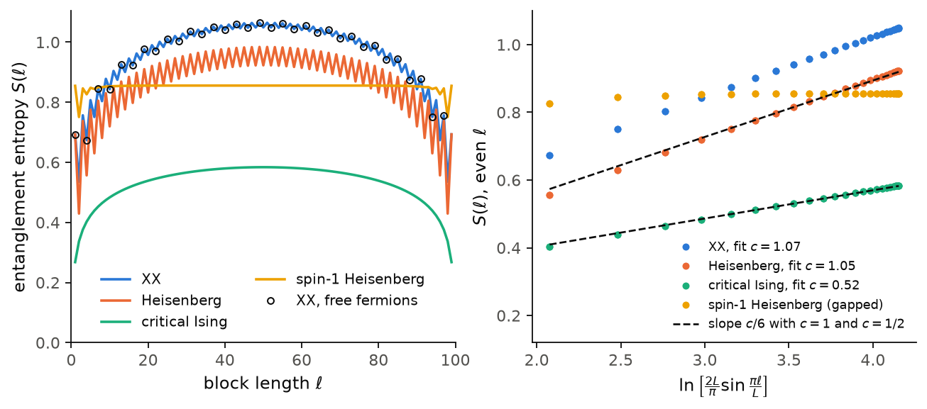
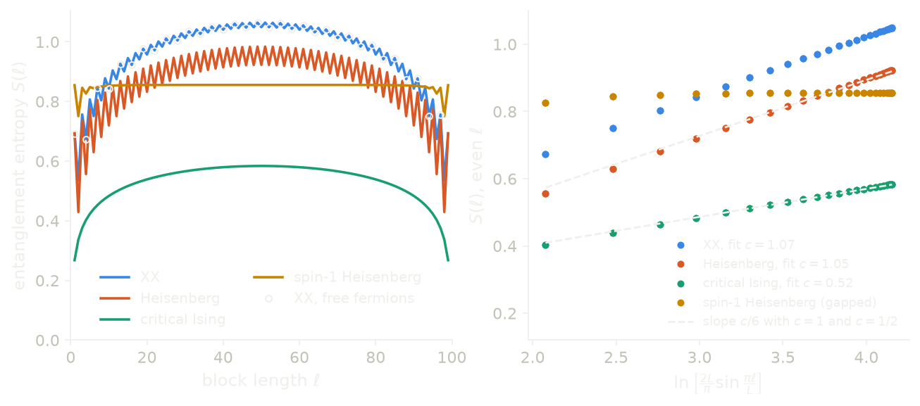
The figure shows open chains with \(L=100\) sites. On the left is the entropy of every cut. For the XX chain the DMRG entropies lie on the exact free-fermion values (circles). The XX, Heisenberg and critical Ising chains follow an arch. For the XX and Heisenberg chains the even-odd oscillation of the open chain sits on top of it. The gapped spin-1 chain is flat in the bulk: its entropy saturates. On the right, the even bonds lie on straight lines against the Calabrese-Cardy variable. The XX and Heisenberg lines are parallel, with \(c\approx1\), and the Ising line has half their slope, \(c\approx1/2\). At \(L=100\) the fits give 1.07, 1.05 and 0.52; the exact free-fermion entropies of the XX chain give the same 1.07, so the remaining difference is a finite-size effect.
Code of this figure (docs/figures/entanglement_central_charge/)
# Bond entanglement entropies S(l) of open critical chains (XX, Heisenberg,
# critical Ising) and of the gapped spin-1 Heisenberg chain, with the exact
# XX entropies from free fermions as the reference.
import numpy as np
from dmrgpy import spinchain

L = 100
names = ["xx", "heisenberg", "ising", "spin1"]
maxm = {"xx": 200, "heisenberg": 200, "ising": 120, "spin1": 100}
ell = np.arange(1, L)


def entropies(name):
    sc = spinchain.Spin_Chain(["S=1" if name == "spin1" else "S=1/2"]*L)
    xy = sum(sc.Sx[i]*sc.Sx[i+1] + sc.Sy[i]*sc.Sy[i+1] for i in range(L-1))
    zz = sum(sc.Sz[i]*sc.Sz[i+1] for i in range(L-1))
    if name == "xx":
        h = xy
    elif name == "ising":
        h = zz + 0.5*sum(sc.Sx[i] for i in range(L))  # critical field
    else:
        h = xy + zz
    sc.set_hamiltonian(h)
    sc.maxm, sc.nsweeps, sc.cutoff = maxm[name], 20, 1e-12
    wf = sc.get_gs()
    return [wf.get_bond_entropy(i, i+1) for i in range(L-1)]


entropy = [entropies(name) for name in names]

# exact XX chain: free fermions with hopping 1/2 at half filling, S(l) from
# the eigenvalues nu of the correlation matrix restricted to the block
hop = 0.5*(np.eye(L, k=1) + np.eye(L, k=-1))
occ = np.linalg.eigh(hop)[1][:, :L//2]
cmat = occ @ occ.T
s_exact = []
for l in ell:
    nu = np.clip(np.linalg.eigvalsh(cmat[:l, :l]), 1e-15, 1-1e-15)
    s_exact.append(-np.sum(nu*np.log(nu) + (1-nu)*np.log(1-nu)))

np.savez("data.npz", L=L, names=names, ell=ell, entropy=entropy,
         s_exact=s_exact)
import numpy as np
import style

d = np.load("data.npz")
L, ell, S = int(d["L"]), d["ell"], d["entropy"]
names = [str(a) for a in d["names"]]
labels = {"xx": "XX", "heisenberg": "Heisenberg", "ising": "critical Ising",
          "spin1": "spin-1 Heisenberg"}
# Calabrese-Cardy, S = c/6 x + const, fitted on even l from 4 to L-4
x = np.log(2*L/np.pi*np.sin(np.pi*ell/L))
even = (ell % 2 == 0) & (ell >= 4) & (ell <= L-4)
c_even = [6*np.polyfit(x[even], s[even], 1)[0] for s in S]
c_exact = 6*np.polyfit(x[even], d["s_exact"][even], 1)[0]  # quoted in the guide


def draw(theme):
    c = style.colors(theme)
    fig, (a, b) = style.figure(2)
    for k, name in enumerate(names):
        a.plot(ell, S[k], "-", color=c["series"][k], label=labels[name])
    a.plot(ell[::3], d["s_exact"][::3], "o", mfc="none", mec=c["ink"],
           ms=4, mew=0.9, label="XX, free fermions")
    a.set_xlabel(r"block length $\ell$")
    a.set_ylabel(r"entanglement entropy $S(\ell)$")
    a.set_xlim(0, L)
    a.set_ylim(bottom=0)
    a.legend(loc="lower center", ncol=2)

    xs = np.linspace(x[even].min(), x[even].max(), 2)
    for k, name in enumerate(names):
        lab = ("%s (gapped)" % labels[name] if name == "spin1" else
               r"%s, fit $c=%.2f$" % (labels[name], c_even[k]))
        b.plot(x[even], S[k][even], "o", color=c["series"][k], ms=3.5,
               label=lab)
    for name, slope in (("heisenberg", 1/6), ("ising", 1/12)):
        s = S[names.index(name)][even]
        b.plot(xs, slope*xs + np.mean(s - slope*x[even]),
               **style.reference(theme),
               label=r"slope $c/6$ with $c=1$ and $c=1/2$"
               if name == "heisenberg" else None)
    b.set_xlabel(r"$\ln\left[\frac{2L}{\pi}\sin\frac{\pi\ell}{L}\right]$")
    b.set_ylabel(r"$S(\ell)$, even $\ell$")
    b.set_ylim(0.12, 1.1)
    b.legend(loc="lower right", fontsize=8)
    return fig


style.main(draw, "entanglement_central_charge")
Participation entropy
A measurement of every site in the computational basis (\(S^z\) for spins, the occupation for fermions) gives a snapshot \(s\) with probability \(p(s)=|\langle s|\psi\rangle|^2\). Snapshots are what a quantum gas microscope or a Rydberg array records. The Rényi participation entropies
measure how much the state spreads over the basis. They grow linearly with the length of the chain. We build \(p(s)\) as an MPS, the elementwise product of \(\psi^*\) and \(\psi\), by recursive sketched interpolation (Meng, Khoo, Li and Stoudenmire, arXiv:2602.17974), whose cost grows as \(\chi^3\), against \(\chi^4\) for the exact product followed by a compression. The sum \(\sum_s p(s)^q\) is then an overlap.
s2 = sc.get_participation_entropy(q=2)             # of the ground state
s3 = sc.get_participation_entropy(wf, q=3, maxm=80)
q: an integer, at least 2.maxm: the bond dimension of \(p\) (default the chain'smaxm). \(p\) needs more than \(\psi\) itself, so check that the result is converged in it.mode="ED": the exact value, for a small chain.
In examples/entanglement/participation_entropy the ground state of the
Heisenberg chain from 4 to 12 sites agrees with ED to \(10^{-7}\), the
accuracy of its own DMRG state.
Single-particle correlation matrix
For fermions, the correlation matrix is
Its eigenvalues \(n_\alpha\in[0,1]\) are the occupations of the natural orbitals. For a single Slater determinant every \(n_\alpha\) is 0 or 1. Interactions move them away from 0 and 1, and the correlation entropy measures how far the state is from a single Slater determinant:
Here fc is a fermionic chain with its Hamiltonian set.
cm = fc.get_correlation_matrix()          # C_ij
na = fc.get_correlation_eigenvalues()     # n_alpha
s = fc.get_correlation_entropy()          # S
orb = fc.get_correlated_orbitals()        # |orbital|^2, most correlated first
rho = fc.get_correlated_density(n=2)      # weight of the 2 most correlated orbitals
sd = fc.get_gs().get_correlation_entropy_density()   # S resolved by site
The most correlated orbitals are those with \(n_\alpha\) closest to \(1/2\). The four-point correlators and the two-particle density matrix are on the Correlators and distributions page. The keywords are:
T: temperature ofget_correlation_matrix(default 0). Finite \(T\) is computed with exact eigenstates, for small chains.dmmode: how \(C_{ij}\) is computed ("fast","full","explicit","simple"). The default chooses the fastest one for the state."explicit"works on every backend.
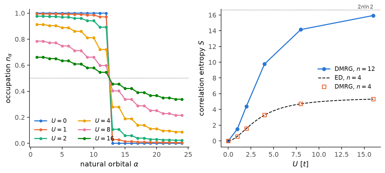
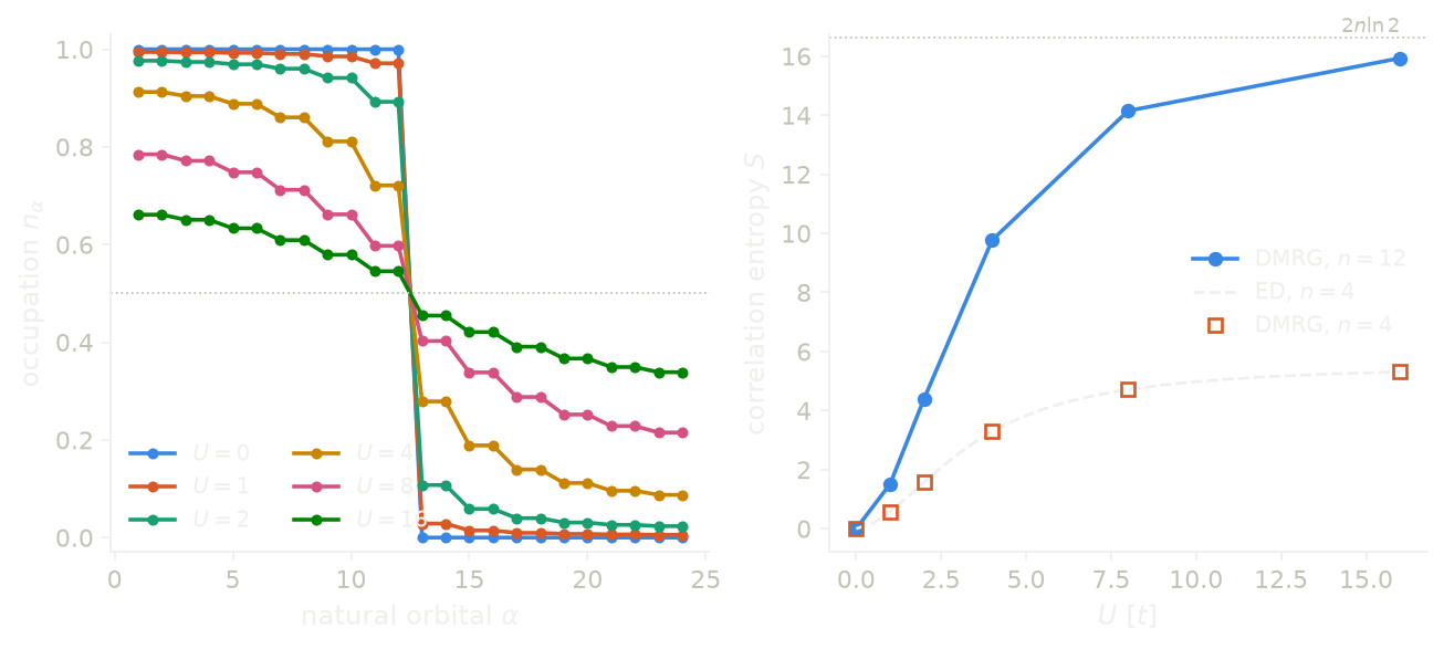
The figure shows the half-filled Hubbard chain with \(n=12\) sites and hopping \(t=1\). On the left are the occupations \(n_\alpha\) for several values of \(U\). At \(U=0\) the ground state is one Slater determinant, so half of the occupations are 1 and the other half are 0. As \(U\) grows, the step melts and all occupations move towards \(1/2\). On the right is the correlation entropy. It starts at zero and grows towards its maximum \(2n\log 2\). For a chain with \(n=4\) the DMRG values (squares) lie on the ED curve (dashed line).
Code of this figure (docs/figures/entanglement_natural_orbitals/)
# Natural-orbital occupations n_alpha and correlation entropy S of the
# half-filled open Hubbard chain as U grows, with ED of a 4-site chain as the
# check of S(U).
import numpy as np
from dmrgpy import fermionchain

n, n_small = 12, 4
Us = [0, 1, 2, 4, 8, 16]
U_fine = np.linspace(0, 16, 33)


def hubbard(nsite, U):
    fc = fermionchain.Spinful_Fermionic_Chain(nsite)
    h = -sum(cd[i]*c[i+1] + cd[i+1]*c[i] for i in range(nsite-1)
             for c, cd in ((fc.Cup, fc.Cdagup), (fc.Cdn, fc.Cdagdn)))
    if U != 0:
        h = h + U*sum(fc.Nup[i]*fc.Ndn[i] for i in range(nsite))
    fc.set_hamiltonian(h)
    fc.set_conserved_sector(Nf=nsite)  # half filling
    fc.maxm, fc.nsweeps = 100, 24
    return fc


occ, s, s_small_dmrg = [], [], []
for U in Us:
    fc = hubbard(n, U)
    occ.append(np.sort(fc.get_correlation_eigenvalues().real)[::-1])
    s.append(fc.get_correlation_entropy())
    s_small_dmrg.append(hubbard(n_small, U).get_correlation_entropy())
s_fine_ed = [hubbard(n_small, U).get_correlation_entropy(mode="ED")
             for U in U_fine]

np.savez("data.npz", n=n, n_small=n_small, U=Us, occ=occ, s=s,
         s_small_dmrg=s_small_dmrg, U_fine=U_fine, s_fine_ed=s_fine_ed)
import numpy as np
import style

d = np.load("data.npz")
n, n_small, U = d["n"], d["n_small"], d["U"]


def draw(theme):
    c = style.colors(theme)
    fig, (a, b) = style.figure(2)
    for k, u in enumerate(U):
        a.plot(np.arange(1, 2*n+1), d["occ"][k], "o-", ms=3.5,
               color=c["series"][k], label=r"$U=%g$" % u)
    a.axhline(0.5, color=c["ink2"], lw=0.8, ls=":")
    a.set_xlabel(r"natural orbital $\alpha$")
    a.set_ylabel(r"occupation $n_\alpha$")
    a.set_ylim(-0.03, 1.03)
    a.legend(loc="lower left", ncol=2)

    b.plot(U, d["s"], "o-", color=c["series"][0], label=r"DMRG, $n=%d$" % n)
    b.plot(d["U_fine"], d["s_fine_ed"], **style.reference(theme),
           label=r"ED, $n=%d$" % n_small)
    b.plot(U, d["s_small_dmrg"], "s", mfc="none", color=c["series"][1],
           mew=1.2, label=r"DMRG, $n=%d$" % n_small)
    b.axhline(2*n*np.log(2), color=c["ink2"], lw=0.8, ls=":")
    b.text(U[-1], 2*n*np.log(2), r"$2n\ln 2$", color=c["ink2"],
           ha="right", va="bottom", fontsize=8)
    b.set_xlabel(r"$U$ [$t$]")
    b.set_ylabel(r"correlation entropy $S$")
    b.legend(loc="center right")
    return fig


style.main(draw, "entanglement_natural_orbitals")