Infinite chains
An infinite chain repeats a unit cell of n_uc sites forever in both
directions. It describes the thermodynamic limit directly, with no edges
and no finite-size extrapolation. The state is a uniform matrix product
state, and the results are densities per site and correlators at any
distance.
Building the Hamiltonian
Each operator exists in three copies per
site i of the unit cell: SzC[i] in the central cell, SzR[i] in the
next cell and SzL[i] in the previous cell. A term is written once, and
it is repeated in every cell:
from dmrgpy import infinitechain
ic = infinitechain.Infinite_Spin_Chain(["1/2"])          # n_uc = 1
h = ic.SxC[0]*ic.SxR[0] + ic.SyC[0]*ic.SyR[0] + ic.SzC[0]*ic.SzR[0]
ic.set_hamiltonian(h)
e = ic.gs_energy()      # energy per site
A two-site cell describes for example a dimerized chain:
ic = infinitechain.Infinite_Spin_Chain(["1/2", "1/2"])
h = (1.0*(ic.SxC[0]*ic.SxC[1] + ic.SyC[0]*ic.SyC[1] + ic.SzC[0]*ic.SzC[1])
     + 0.4*(ic.SxC[1]*ic.SxR[0] + ic.SyC[1]*ic.SyR[0] + ic.SzC[1]*ic.SzR[0]))
ic.set_hamiltonian(h)
For longer couplings, ic.get_operator(name, i, group=c) gives site i
of the cell at distance c, so c=-1,0,1 are L, C, R. For example
a J1-J2 chain on a one-site cell:
h = 0
for op in ("Sx", "Sy", "Sz"):
    o0 = ic.get_operator(op, 0)
    h = h + o0*ic.get_operator(op, 0, group=1)        # J1
    h = h + 0.4*o0*ic.get_operator(op, 0, group=2)    # J2
At \(J_2=0.4\) this chain is dimerized, so its ground state has a period of two sites. A one-site cell cannot hold it and the solver does not converge. Use the same couplings on a two-site cell for this phase.
Fermionic chains use Infinite_Many_Body_Chain with a list of site
codes: 0 for a spinless fermion (C, Cdag, N) and 1 for a
spinful site (Cup, Cdagup, Cdn, Cdagdn, Nup, Ndn). The
Jordan-Wigner string is added automatically, also for hoppings that skip
sites. A term with an odd number of fermion operators raises an error.
Two solvers
ic.gs_method selects the algorithm:
"vumps"(the default): variational uniform MPS (arXiv:1701.07035). It finds the best state of bond dimensionmaxmdirectly in the thermodynamic limit. It works for any unit cell and any range of coupling."idmrg": infinite DMRG, which grows a finite chain from the center until the energy per site converges. Onlyn_ucof 1 or 2.
Both run on itensor_version="python" and 3. On "julia_live",
"vumps" runs for n_uc of 1 or 2 with couplings between neighboring
cells, for the energy, vev and correlator; everything else raises an
error there, and so does itensor_version=2. The keywords are:
ic.maxm,ic.cutoff: the bond dimension (default 30) and the truncation cutoff. Increasemaxmuntil the results stop changing.ic.maxiter,ic.etol: the maximal number of iterations and the energy tolerance.ic.vumps_nrestarts: the number of random starts of VUMPS (default 4).ic.noise,ic.noise_iters: for iDMRG. A particle-conserving model has the empty and the full state as exact eigenstates, and iDMRG can get stuck in them. The noise (default \(10^{-4}\)) breaks this, and is applied only while the state is a product state.
After the solve, ic.converged says whether the tolerance was reached.
If it was not, gs_energy() also gives a RuntimeWarning with the
reason. VUMPS starts from a random state, so on a hard model
call gs_energy() a few times and keep the lowest energy. A simple
product state, such as the Neel state, gives an upper bound to compare
with. For a gapless
model on a one-site cell, iDMRG can end in a dimerized state (see
Static correlators). Then the energy per site
alternates between iterations, so converged stays False while the
energy is already accurate to several digits. Entanglement
entropies are not available for infinite chains.
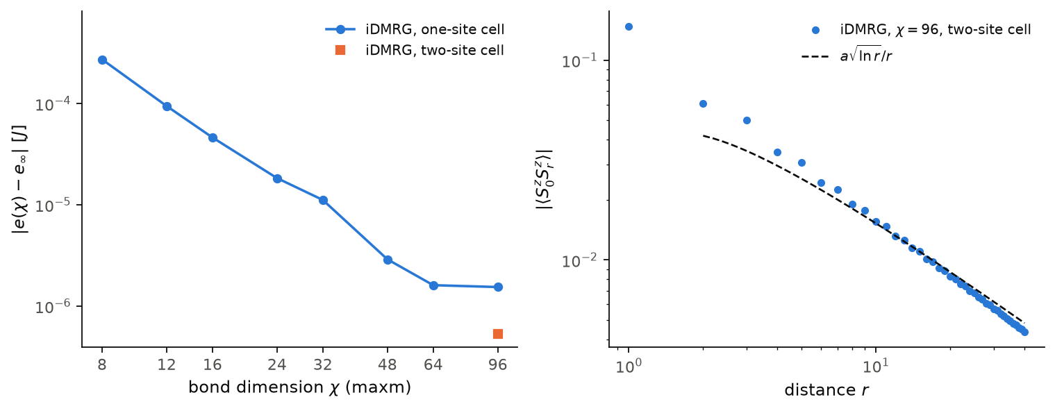
The left panel shows the error of the iDMRG energy per site of the
spin-1/2 Heisenberg chain, against the Bethe-ansatz value
\(e_\infty=1/4-\ln 2\), as a function of maxm. The chain is gapless, so
the error falls as a power of maxm, from \(3\times10^{-4}\) at maxm=8
to \(1.6\times10^{-6}\) at maxm=64. On the one-site cell it stops there.
A two-site cell gives \(5\times10^{-7}\) at maxm=96 (square). Here
converged stays False up to maxm=64, because the one-site state is
dimerized, while the energy is already accurate. The right panel is described in
Static correlators.
Code of this figure (docs/figures/infinite-chains_energy/)
# Energy per site of the infinite spin-1/2 Heisenberg chain against the bond
# dimension (iDMRG), and the spin correlator at long distance.
import numpy as np
from dmrgpy import infinitechain

maxms = [8, 12, 16, 24, 32, 48, 64, 96]
rmax = 40
e_exact = 0.25 - np.log(2)  # Bethe ansatz


def heisenberg(cell, m):
    ic = infinitechain.Infinite_Spin_Chain(cell)
    h = 0
    for o in ("Sx", "Sy", "Sz"):
        oc, orr = getattr(ic, o + "C"), getattr(ic, o + "R")
        if len(cell) == 1:
            h = h + oc[0]*orr[0]
        else:
            h = h + oc[0]*oc[1] + oc[1]*orr[0]
    ic.set_hamiltonian(h)
    ic.gs_method, ic.maxm, ic.maxiter, ic.etol = "idmrg", m, 400, 1e-10
    return ic


energy, converged = [], []
for m in maxms:
    ic = heisenberg(["1/2"], m)
    energy.append(ic.gs_energy())
    converged.append(bool(ic.converged))

# At finite maxm the iDMRG state of this critical chain alternates between
# strong and weak bonds, so the correlator is taken on a two-site cell and
# averaged over its two sites.
ic2 = heisenberg(["1/2", "1/2"], maxms[-1])
e_uc2 = ic2.gs_energy()
r = np.arange(1, rmax + 1)
czz = np.mean([[ic2.correlator("Sz", i, "Sz", int(x)).real for x in r]
               for i in (0, 1)], axis=0)

np.savez("data.npz", maxm=maxms, energy=energy, converged=converged,
         e_exact=e_exact, e_uc2=e_uc2, r=r, czz=czz)
import numpy as np
import style

d = np.load("data.npz")
maxm, r = d["maxm"], d["r"]
err = np.abs(d["energy"] - d["e_exact"])
err_uc2 = abs(d["e_uc2"] - d["e_exact"])
c = np.abs(d["czz"])
# Luttinger form a sqrt(ln r)/r, a fitted in log space on r = 8 to 20
fit = (r >= 8) & (r <= 20)
a = np.exp(np.mean(np.log(c[fit]) - np.log(np.sqrt(np.log(r[fit]))/r[fit])))
rr = np.linspace(2, r.max(), 200)


def draw(theme):
    col = style.colors(theme)
    fig, (ax1, ax2) = style.figure(2)
    ax1.plot(maxm, err, "o-", color=col["series"][0],
             label="iDMRG, one-site cell")
    ax1.plot([maxm[-1]], [err_uc2], "s", color=col["series"][1],
             label="iDMRG, two-site cell")
    ax1.set_xscale("log")
    ax1.set_yscale("log")
    ax1.set_xticks(maxm)
    ax1.set_xticklabels([str(m) for m in maxm])
    ax1.minorticks_off()
    ax1.set_xlabel(r"bond dimension $\chi$ (maxm)")
    ax1.set_ylabel(r"$|e(\chi)-e_\infty|$ [$J$]")
    ax1.legend()
    ax1.set_ylim(top=err.max()*3)

    ax2.plot(r, c, "o", color=col["series"][0], ms=4,
             label=r"iDMRG, $\chi=%d$, two-site cell" % maxm[-1])
    ax2.plot(rr, a*np.sqrt(np.log(rr))/rr, **style.reference(theme),
             label=r"$a\sqrt{\ln r}/r$")
    ax2.set_xscale("log")
    ax2.set_yscale("log")
    ax2.set_xlabel(r"distance $r$")
    ax2.set_ylabel(r"$|\langle S^z_0S^z_r\rangle|$")
    ax2.legend()
    fig.tight_layout()
    return fig


style.main(draw, "infinite-chains_energy")
Static correlators
ic.vev("Sz", 0)                    # <Sz> on site 0 of the cell
ic.correlator("Sz", 0, "Sz", r)    # <Sz_0 Sz_r>, r in sites, r >= 0
ic.correlator("Cdag", 0, "C", r)   # fermionic chain, with the string
They work with both solvers and both backends. A pair with an odd number
of fermion operators raises an error. A good check of maxm needs no
reference value: the sum of the bond correlators of one unit cell must be
equal to n_uc times the energy per site.
With iDMRG at finite maxm, a gapless chain can end in a dimerized
state: the bonds alternate in strength. This comes from the finite
maxm, and the alternation becomes smaller when maxm grows. A one-site
cell cannot hold this state. The energy per site then alternates between
iterations, so converged stays False, and
ic.correlator("Sz", 0, "Sz", 1) gives only one of the two bonds. In
this case gs_energy, vev and correlator give a RuntimeWarning
with the entanglement entropies of the two bonds. On a two-site cell both
bonds are measured, and their mean is the energy per site.
When VUMPS did not converge, vev, correlator and the excitations also
give a RuntimeWarning. Such a state is not a consistent uniform MPS, and
its correlators can be wrong by 10 per cent while its energy is accurate.
The right panel of the figure in Two solvers shows
\(|\langle S^z_0S^z_r\rangle|\) of the Heisenberg chain on a two-site
cell at maxm=96, averaged over the two sites. There is no edge, so the
correlator decays as the power law \(a\sqrt{\ln r}/r\) of a Luttinger
liquid (dashed, \(a\) fitted at \(r=8\) to 20). At \(r=1\) it gives
\(3\langle S^z_0S^z_1\rangle=-0.443147\), which is \(e_\infty\). At the
largest \(r\) the data fall a little below the power law, because a finite
maxm gives a finite correlation length.
Excitations
In an infinite chain the excitations form bands \(E(k)\). We use the quasiparticle ansatz: one tensor \(B\) inserted on top of the ground state, in a plane wave of momentum \(k\). This gives the dispersion of the lowest modes, as measured by inelastic neutron scattering:
ic.excitation_energies(k, n=1)   # n lowest energies at momentum k
ic.excitation_gap()              # minimum over k
\(k\) is in radians per unit cell. It needs gs_method="vumps", n_uc of
1 or 2, and couplings to the neighboring cell only.
Dynamical structure factor
Each quasiparticle branch \(a\) contributes a delta peak to \(S(k,\omega)\) with weight \(w_a=|\langle k,a|O_k|\mathrm{GS}\rangle|^2\):
e, w = ic.spectral_weights("Sz", k, n=2)
e, w, total = ic.spectral_weights("Sz", k, n=2, return_total=True)
ks, es, S = ic.dynamical_structure_factor("Sz", delta=0.05)  # map in (k, w)
The peaks are exact in momentum and energy. They do not contain the
continuum of two or more particles. total is the static structure
factor \(\sum_re^{ikr}(\langle O_0O_r\rangle-\langle O\rangle^2)\), so
w.sum()/total is the fraction of the weight in the computed branches.
When it is close to 1, a single-mode picture is valid at that \(k\). In
dynamical_structure_factor, delta is a Lorentzian broadening for
plotting. These two methods need gs_method="vumps" and a parity-even
operator, on itensor_version="python" or 3. See
examples/idmrg/dynamical_structure_factor_tfim.
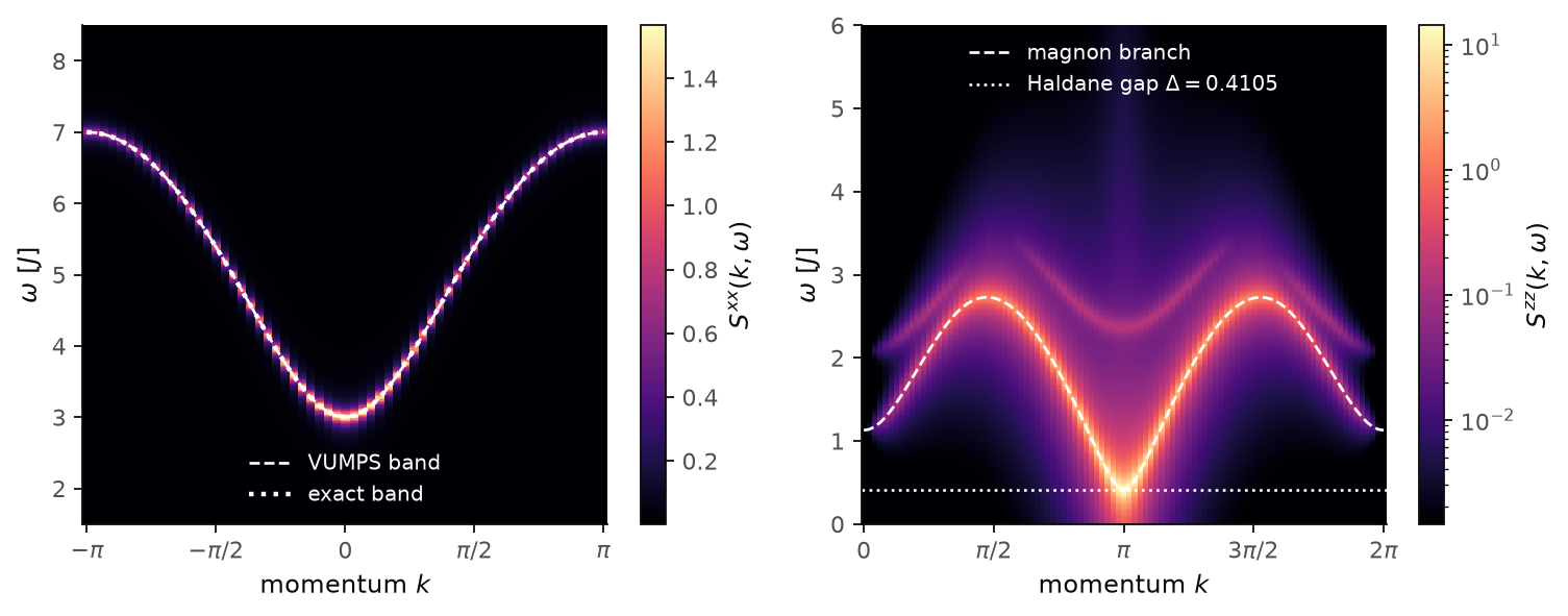
The left panel is the transverse-field Ising chain
\(H=-\sum\sigma^x\sigma^x-g\sum\sigma^z\) at \(g=2.5\), in the paramagnetic
phase, with maxm=4. The map is \(S^{xx}(k,\omega)\). The VUMPS band
(dashed) lies on the exact free-fermion band
\(2\sqrt{1+g^2-2g\cos k}\) (dotted) within \(10^{-8}\). The right panel is
the spin-1 Heisenberg chain with maxm=16, and the map is
\(S^{zz}(k,\omega)\) on a log color scale. The magnon branch has its
minimum at \(k=\pi\). There it gives the Haldane gap \(0.4098\), against the
reference \(0.4105\) (dotted line). Near \(k=0\) the weight goes to zero,
because \(\sum_jS^z_j\) is conserved. The weak features above the branch
come from higher states of the ansatz. The ansatz does not describe the
two-magnon continuum, which starts at \(2\Delta\).
Code of this figure (docs/figures/infinite-chains_excitations/)
# Excitation bands of infinite chains from the quasiparticle ansatz on top of
# VUMPS, with the dynamical structure factor S(k,omega) of the same ansatz:
# (a) the transverse-field Ising chain, (b) the spin-1 Heisenberg chain.
import numpy as np
from dmrgpy import infinitechain


def vumps_chain(spin, h, maxm):
    ic = infinitechain.Infinite_Spin_Chain([spin], itensor_version="python")
    ic.set_hamiltonian(h(ic))
    ic.gs_method, ic.maxm = "vumps", maxm
    ic.maxiter, ic.vumps_nrestarts = 800, 6
    ic.gs_energy()
    return ic


# (a) H = -sum sx sx - g sum sz in Pauli matrices, paramagnetic phase
g = 2.5
ic = vumps_chain("1/2", lambda c: -4.0*c.SxC[0]*c.SxR[0] - 2.0*g*c.SzC[0], 4)
ks_a = np.linspace(-np.pi, np.pi, 61)
band_a = np.array([ic.excitation_energies(k, n=1)[0] for k in ks_a]).real
exact_a = 2*np.sqrt(1 + g**2 - 2*g*np.cos(ks_a))  # free-fermion band
_, es_a, S_a = ic.dynamical_structure_factor(
    "Sx", ks=ks_a, energies=np.linspace(1.5, 8.5, 400), delta=0.08, n=1)

# (b) spin-1 Heisenberg chain, 12 branches of the ansatz at each k
ich = vumps_chain("1", lambda c: c.SxC[0]*c.SxR[0] + c.SyC[0]*c.SyR[0]
                  + c.SzC[0]*c.SzR[0], 16)
ks_b = np.linspace(0, 2*np.pi, 97)
e_b, w_b = [], []
for k in ks_b:
    # energies E_a(k) and weights |<k,a|S^z_k|GS>|^2
    e, w = ich.spectral_weights("Sz", k, n=12)
    e_b.append(np.real(e))
    w_b.append(np.real(w))
e_b, w_b = np.array(e_b), np.array(w_b)
es_b, delta = np.linspace(0, 6, 400), 0.08
lorentz = (delta/np.pi)/((es_b[None, :, None] - e_b[:, None, :])**2 + delta**2)
S_b = np.einsum("kea,ka->ke", lorentz, w_b)
gap_ref = 0.4104789  # Haldane gap

np.savez("data.npz", ks_a=ks_a, band_a=band_a, exact_a=exact_a, es_a=es_a,
         S_a=np.real(S_a), ks_b=ks_b, e_b=e_b, es_b=es_b, S_b=S_b,
         gap_ref=gap_ref)
import numpy as np
from matplotlib.colors import LogNorm
import style

d = np.load("data.npz")
ks_a, es_a, S_a = d["ks_a"], d["es_a"], d["S_a"]
ks_b, es_b, S_b = d["ks_b"], d["es_b"], d["S_b"]
band_b, gap = d["e_b"][:, 0], float(d["gap_ref"])
PI_NAMES = {0: "0", 1: r"$\pi/2$", -1: r"$-\pi/2$", 2: r"$\pi$", -2: r"$-\pi$",
            3: r"$3\pi/2$", 4: r"$2\pi$"}


def pi_ticks(ax, k):
    q = np.pi/2
    t = np.arange(np.ceil(k[0]/q - 1e-9), np.floor(k[-1]/q + 1e-9) + 1)
    ax.set_xticks(t*q)
    ax.set_xticklabels([PI_NAMES[int(v)] for v in t])


def draw(theme):
    fig, (ax1, ax2) = style.figure(2)
    im = ax1.pcolormesh(ks_a, es_a, S_a.T, shading="auto", cmap=style.CMAP,
                        rasterized=True)
    ax1.plot(ks_a, d["band_a"], **style.heatmap_line(), label="VUMPS band")
    ax1.plot(ks_a, d["exact_a"], color="white", ls=":", lw=2.0,
             label="exact band")
    ax1.legend(loc="lower center", labelcolor="white")
    style.colorbar(fig, im, ax1, r"$S^{xx}(k,\omega)$", theme)

    vmax = S_b.max()
    im = ax2.pcolormesh(ks_b, es_b, np.maximum(S_b.T, 1e-12), shading="auto",
                        cmap=style.CMAP, rasterized=True,
                        norm=LogNorm(vmin=1e-4*vmax, vmax=vmax))
    ax2.plot(ks_b, band_b, **style.heatmap_line(), label="magnon branch")
    ax2.axhline(gap, color="white", ls=":", lw=1.2,
                label=r"Haldane gap $\Delta=%.4f$" % gap)
    ax2.legend(loc="upper center", labelcolor="white")
    style.colorbar(fig, im, ax2, r"$S^{zz}(k,\omega)$", theme)
    for ax, k in ((ax1, ks_a), (ax2, ks_b)):
        pi_ticks(ax, k)
        ax.set_xlabel(r"momentum $k$")
        ax.set_ylabel(r"$\omega$ [$J$]")
    fig.tight_layout()
    return fig


style.main(draw, "infinite-chains_excitations")
Local gap estimate
ic.local_excitation_gap() takes the converged
two-site block of iDMRG and returns the gap between its two lowest
states. It is cheap, but less accurate than excitation_gap() (10 per
cent too high on the XX chain). On fermionic models it can be a charge
excitation and shifts with a uniform chemical potential. Use it only as a
rough check. It needs gs_method="idmrg". window=w, with
itensor_version="python" and n_uc=1, adds w sites on each side of
the block and improves the estimate.
Dynamical correlators
Two methods compute \(\langle O_i(t)O_j\rangle\) and its spectrum in an infinite chain:
es, ys = ic.kpm_finite("Sz", 0, "Sz", 0, n_window=16,
             window_chain_kwargs=dict(maxm=30, nsweeps=15),
             delta=0.3, es=np.linspace(-1, 5, 200))
ic.gs_method = "idmrg"
ks, es, Skw = ic.td_dynamical_correlator("Sz", 0, "Sz", n_window=14,
             dt=0.05, nt=200, maxdim=60, x_values=range(-6, 7),
             ks=np.linspace(-np.pi, np.pi, 41), delta=0.1)
kpm_finite: the KPM dynamical correlator on a finite open window ofn_windowunit cells. It has finite-size and edge effects, so converge it inn_window. A smalldeltaneeds many moments, and then the edges matter even for a long window. The window runs on the same backend as the infinite chain.td_dynamical_correlator: real-time evolution of a window whose two ends are attached to the converged infinite environment (arXiv:1804.09163), so it has no edges. One evolution gives every distancexand every momentumk.n_windowandx_valuesmust be converged separately. It needsgs_method="idmrg".connected=True(default) subtracts \(\langle O_i\rangle\langle O_j\rangle\). It returns the one-sided Fourier transform, so take the real part ofSkwfor the spectral function.
See examples/idmrg/td_dynamical_correlator for both.
Operators on the state, overlaps and sums
Three methods act on the converged state itself and return the result as
a new chain, so that vev and correlator measure it. Here ic and
ic2 are two converged chains on the same unit cell. They run on
itensor_version="python" with both solvers, and on itensor_version=3
with gs_method="vumps":
flipped = ic.apply_operator(2*ic.SxC[0])   # Pauli X on every site
flipped.vev("Sz", 0)                       # -<Sz> of ic
flipped.eta                                # 1 for a unitary operator
f = ic.overlap(flipped)                    # fidelity per site, 0 to 1
f2 = ic.overlap(ic2)                       # between two solved chains
try:
    cat = ic.summps(ic2)                   # |ic> + |ic2>
except RuntimeError:
    pass                                   # two normalized states, see below
apply_operator(op):opis an operator on the central cell, built fromic.SxC,ic.SzC[0]*ic.SzC[1]and so on, applied in every cell at once. It must stay inside the cell (anSxRfactor raises an error), since it is repeated cell by cell. The state is normalized afterwards, andetais the factor by which the operator changed its norm per cell. A gate that entangles neighboring sites grows the bond dimension, and the result is refused when truncating it back loses weight; passmaxdim=larger thanic.maxm. The gauge fixing behind this holds only for a state solved at a modestmaxm(4 worked, 8 did not, on a free-fermion cell), so apply such a gate to a small state.overlap(other): the fidelity per site of two states on the same unit cell, \(|\langle\phi|\psi\rangle|^{1/N}\) in the limit of \(N\) sites. It is 1 for the same physical state in any gauge, and below 1 otherwise. Two ground states on the two sides of a phase transition have a fidelity that drops at the transition, the infinite-chain version of Fidelity susceptibility.summps(other): the direct sum of two states. Tiled to infinity, the sum keeps only the branch of larger norm per site, so two normalized ground states tie and raise an error: a cat state of two ordered states has no uniform MPS representation.
The returned chain is not a ground state, so gs_energy() and the
excitations raise on it; set_hamiltonian() makes it an ordinary chain
again. See examples/idmrg/apply_mpo_to_infinite_chain and
examples/idmrg/imps_overlap.