DMRGPY
DMRGPY is a Python library for quasi-one-dimensional quantum many-body systems: spin chains, spinless and spinful fermions, bosons and parafermions. Ground states, excitations, dynamical correlators, real-time evolution and finite temperature are computed with matrix product states. Small systems can also be solved with exact diagonalization (ED), so every DMRG result can be checked on a short chain.
This guide explains how to compute physical quantities. For each capability it gives the quantity, its formula, the code and the keywords that matter. The code itself is on GitHub, and the whole guide is also available as one PDF.
Installation
pip install dmrgpy
This installs ED and a DMRG code written in pure Python. It needs no
compiler and works on Linux, Mac and Windows. The faster C++ backend
(ITensor) is compiled from a clone of the repository with
python install.py; the
README explains how.
A first calculation
The ground-state energy of a spin-1/2 Heisenberg chain of 12 sites, with DMRG and with ED:
from dmrgpy import spinchain
n = 12
sc = spinchain.Spin_Chain(["S=1/2" for i in range(n)])
h = sum(sc.Sx[i]*sc.Sx[i+1] + sc.Sy[i]*sc.Sy[i+1] + sc.Sz[i]*sc.Sz[i+1]
        for i in range(n-1))
sc.set_hamiltonian(h)
print(sc.gs_energy())            # DMRG
print(sc.gs_energy(mode="ED"))   # exact diagonalization
Both print \(E_0\approx-5.1420906\). Every chain class has the same methods,
and most of them accept mode="ED" in the same way.
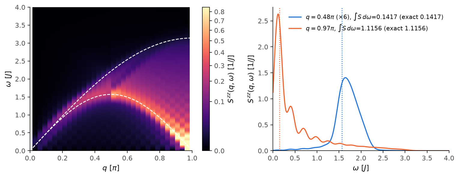
A Heisenberg chain with \(n=32\) gives the dynamical spin structure factor \(S(q,\omega)\), the quantity measured by inelastic neutron scattering. The weight fills the two-spinon continuum between its exact edges (dashed). See Dynamical correlators.
Code of this figure (docs/figures/dynamical-correlators_sqw/)
# Dynamical spin structure factor S^zz(q,w) of the open spin-1/2 Heisenberg
# chain, one KPM run per momentum. On an open chain the momentum states are
# standing waves, S^z_q = sqrt(2/(n+1)) sum_i sin(q(i+1)) S^z_i, q = pi k/(n+1).
import numpy as np
from dmrgpy import spinchain, kpmdmrg

n = 32
delta = 0.15
es = np.linspace(0.0, 4.0, 400)
qs = np.pi*np.arange(1, n+1)/(n+1)

sc = spinchain.Spin_Chain(["S=1/2"]*n)
h = sum(sc.Sx[i]*sc.Sx[i+1] + sc.Sy[i]*sc.Sy[i+1] + sc.Sz[i]*sc.Sz[i+1]
        for i in range(n-1))
sc.set_hamiltonian(h)
sc.maxm, sc.nsweeps, sc.cutoff = 80, 14, 1e-12
sc.kpmmaxm = 40  # kpmmaxm=80 changes S(q,w) at q close to pi by less than 1%
sc.gs_energy()


def spectrum(x, mus, emin, emax, scale, npol, d):
    _, y = kpmdmrg.dynamical_correlator_from_moments(
        mus, emin, emax, scale, npol, x, kernel="jackson", delta=d,
        origin=sc.e0)
    return y.real


sqw, sumrule, sq = [], [], []
for q in qs:
    Sq = sum(np.sqrt(2/(n+1))*np.sin(q*(i+1))*sc.Sz[i] for i in range(n))
    m = sc.get_dynamical_correlator_moments(name=(Sq, Sq), delta=delta)
    sqw.append(spectrum(es, *m))
    # sum rule: the integral over the whole spectrum is <S^z_q S^z_q>
    ew = np.linspace(-1.0, m[2] - sc.e0 + 1.0, 20000)
    sumrule.append(np.trapezoid(spectrum(ew, *m), ew))
    sq.append(sc.vev(Sq*Sq).real)

np.savez("data.npz", qs=qs, es=es, sqw=sqw, sumrule=sumrule, sq=sq)
import numpy as np
from matplotlib.colors import PowerNorm
import style

d = np.load("data.npz")
qs, es = d["qs"], d["es"]
sqw = np.clip(d["sqw"], 0.0, None)  # tiny Jackson ringing below zero
# two-spinon continuum edges
qq = np.linspace(0, np.pi, 300)
lower, upper = np.pi/2*np.abs(np.sin(qq)), np.pi*np.abs(np.sin(qq/2))
cuts = [int(np.argmin(np.abs(qs - np.pi/2))), len(qs) - 1]


def draw(theme):
    c = style.colors(theme)
    fig, (a1, a2) = style.figure(2, gridspec_kw={"width_ratios": [1.15, 1]})
    im = a1.pcolormesh(qs/np.pi, es, sqw.T, cmap=style.CMAP, shading="nearest",
                       norm=PowerNorm(0.5, vmin=0, vmax=np.percentile(sqw, 99.5)),
                       rasterized=True)
    a1.plot(qq/np.pi, lower, **style.heatmap_line())
    a1.plot(qq/np.pi, upper, **style.heatmap_line())
    a1.set_xlim(0, 1)
    a1.set_ylim(es[0], es[-1])
    a1.set_xlabel(r"$q$ [$\pi$]")
    a1.set_ylabel(r"$\omega$ [$J$]")
    style.colorbar(fig, im, a1, r"$S^{zz}(q,\omega)$ [$1/J$]", theme)
    big = np.max(sqw[cuts[-1]])
    for k, idx in enumerate(cuts):
        q, col = qs[idx], c["series"][k]
        f = max(1, int(round(0.5*big/np.max(sqw[idx])))) if k == 0 else 1
        a2.plot(es, f*sqw[idx], color=col, lw=style.LW,
                label=r"$q=%.2f\pi$%s, $\int S\,d\omega$=%.4f (exact %.4f)"
                % (q/np.pi, r" ($\times%d$)" % f if f > 1 else "",
                   d["sumrule"][idx], d["sq"][idx]))
        a2.axvline(np.pi/2*np.sin(q), color=col, ls=":", lw=style.LW_REF)
    a2.set_xlim(es[0], es[-1])
    a2.set_ylim(0, None)
    a2.set_xlabel(r"$\omega$ [$J$]")
    a2.set_ylabel(r"$S^{zz}(q,\omega)$ [$1/J$]")
    a2.legend(loc="upper right")
    fig.tight_layout()
    return fig


style.main(draw, "dynamical-correlators_sqw")
Backends
The keyword itensor_version= of a chain chooses the DMRG code. The
results are the same; only the speed and a few features differ.
3: ITensor v3 in C++, the default when it is compiled. The fastest."python": the pure-Python DMRG, the default afterpip install. It can also run on a GPU (Performance).2: ITensor v2 in C++. Some features are missing."julia_live": ITensors.jl in Julia, afterpip install "dmrgpy[julia]".
mode="ED" uses exact diagonalization instead of DMRG, for small chains.
Contents of the guide
- Getting started: the chain classes, their local operators, and how to write a Hamiltonian.
- Ground state: energies, expectation values, correlators and conserved sectors; the solver settings and warm starts; excited states and degeneracies; entanglement; four-point correlators and distributions; mean-field decoupling.
- Phases: Berry phases, fermion parity and the fidelity susceptibility.
- Dynamics: dynamical correlators, spectral functions and the local density of states, real-time evolution and STM spectra.
- Finite temperature: purification, METTS and ED.
- Infinite chains: iDMRG and VUMPS directly in the thermodynamic limit.
- More: the common models written out, post-processing tools and performance.