Post-processing tools
extrapolate.size_extrapolation(L, y, n=1): fits \(y(L)\) with a polynomial of ordernin \(1/L\) and returns the value at \(L\to\infty\). Use it for energy densities, gaps and order parameters from finite chains.
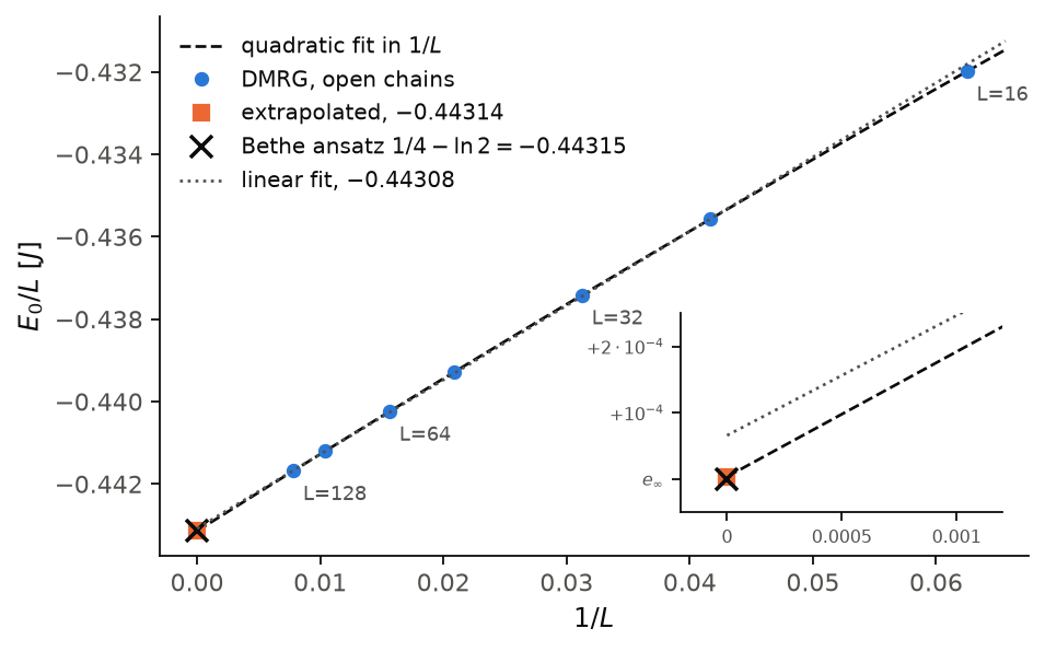
The figure shows the ground-state energy per site of open Heisenberg
chains, from \(L=16\) to \(L=128\), as a function of \(1/L\). On an open chain
the edges add an energy of order one, so \(E_0/L=e_\infty+a/L+b/L^2\). The
quadratic fit (n=2) gives \(e_\infty=-0.443143\), which differs from the
Bethe-ansatz value \(1/4-\ln 2=-0.443147\) by \(4\times10^{-6}\). The linear
fit (n=1) misses the curvature and is more than 15 times worse. The
inset zooms on \(1/L=0\).
Code of this figure (docs/figures/post-processing_extrapolation/)
compute.py
# Energy per site of open spin-1/2 Heisenberg chains against 1/L, extrapolated
# to L -> infinity with extrapolate.size_extrapolation.
import numpy as np
from dmrgpy import spinchain, extrapolate

Ls = np.array([16, 24, 32, 48, 64, 96, 128])

energy = []
for L in Ls:
    sc = spinchain.Spin_Chain(["S=1/2"]*L)
    sc.set_hamiltonian(sum(sc.Sx[i]*sc.Sx[i+1] + sc.Sy[i]*sc.Sy[i+1]
                           + sc.Sz[i]*sc.Sz[i+1] for i in range(L-1)))
    sc.maxm, sc.nsweeps = 100, 16
    energy.append(sc.gs_energy())
energy = np.array(energy)

# E/L = e_inf + a/L (n=1), plus b/L^2 (n=2)
e_inf_n1 = extrapolate.size_extrapolation(Ls, energy/Ls, n=1)
e_inf_n2 = extrapolate.size_extrapolation(Ls, energy/Ls, n=2)
e_exact = 0.25 - np.log(2)  # Bethe ansatz

np.savez("data.npz", L=Ls, energy=energy, e_inf_n1=e_inf_n1,
         e_inf_n2=e_inf_n2, e_exact=e_exact)
plot.py
import numpy as np
from numpy.polynomial import polynomial as P
import style

d = np.load("data.npz")
L = d["L"]
x, y = 1.0/L, d["energy"]/L
e_exact = float(d["e_exact"])
e1, e2 = float(d["e_inf_n1"]), float(d["e_inf_n2"])
# the same weighted fits as extrapolate.size_extrapolation(n=1, 2)
xf = np.linspace(0.0, x.max()*1.05, 200)
yf1, yf = (P.polyval(xf, P.polyfit(x, y, deg, w=L)) for deg in (1, 2))
assert abs(yf1[0] - e1) < 1e-12 and abs(yf[0] - e2) < 1e-12


def draw(theme):
    col = style.colors(theme)
    fig, ax = style.figure(1)
    ax.plot(xf, yf, **style.reference(theme), label="quadratic fit in $1/L$")
    ax.plot(x, y, "o", color=col["series"][0], label="DMRG, open chains")
    ax.plot([0], [e2], "s", color=col["series"][1], ms=6,
            label=r"extrapolated, $%.5f$" % e2)
    ax.plot([0], [e_exact], "x", color=col["ink"], ms=9, mew=1.6,
            label=r"Bethe ansatz $1/4-\ln 2=%.5f$" % e_exact)
    ax.plot(xf, yf1, color=col["ink2"], ls=":", lw=style.LW_REF,
            label=r"linear fit, $%.5f$" % e1)
    for Li, xi, yi in zip(L, x, y):
        if Li in (16, 32, 64, 128):
            ax.annotate("L=%d" % Li, (xi, yi), textcoords="offset points",
                        xytext=(4, -12), fontsize=8, color=col["ink2"])
    ax.set_xlim(-0.003, x.max()*1.08)
    ax.set_xlabel(r"$1/L$")
    ax.set_ylabel(r"$E_0/L$ [$J$]")
    ax.legend(loc="upper left")
    # zoom on the extrapolation
    ins = ax.inset_axes([0.6, 0.08, 0.37, 0.37])
    ins.plot(xf, yf, **style.reference(theme))
    ins.plot(xf, yf1, color=col["ink2"], ls=":", lw=style.LW_REF)
    ins.plot(x, y, "o", color=col["series"][0])
    ins.plot([0], [e2], "s", color=col["series"][1], ms=6)
    ins.plot([0], [e_exact], "x", color=col["ink"], ms=9, mew=1.6)
    ins.set_xlim(-0.0002, 0.0012)
    ins.set_ylim(e_exact - 5e-5, e_exact + 2.5e-4)
    ins.set_xticks([0, 0.0005, 0.001])
    ins.set_xticklabels(["0", "0.0005", "0.001"])
    ins.set_yticks([e_exact, e_exact + 1e-4, e_exact + 2e-4])
    ins.set_yticklabels([r"$e_\infty$", r"$+10^{-4}$", r"$+2\cdot10^{-4}$"])
    ins.tick_params(labelsize=7)
    ins.set_facecolor("none")
    return fig


style.main(draw, "post-processing_extrapolation")
functionfit.fit(f, x0): minimizes a functionfwith several random starts of the Powell method. Use it for fits such as the Calabrese-Cardy formula.analyticcontinuation.imag2real(zs, us): Pade continuation of a function known at complex frequencieszsto the real axis, for example the output ofsubmode="CVMimag"(Choosing a correlator method). The fartherzsis from the real axis, the more the result is smoothed.reconstruct.reconstruct_distribution: maximum-entropy reconstruction of a positive spectral function from its moments, used bysubmode="maxent"andget_distribution_maxent.