Correlators and distributions
On this page we measure the ground state beyond a two-point correlator: four-point correlators, the two-particle density matrix, and the full distribution of an operator. Two-point correlators and the equal-time structure factor are on the Ground state page, and the single-particle correlation matrix, whose eigenvalues are the natural orbitals, is under Entanglement.
Four-point correlators
For a fermionic chain fc, the four-point tensor
\(\langle c_i^\dagger c_jc_k^\dagger c_l\rangle\) for all \(i,j,k,l\) is
t = fc.get_gs().get_four_correlation_tensor() # shape (n, n, n, n)
It holds every density-density correlator \(\langle n_in_k\rangle\) (at
\(j=i\), \(l=k\)) and every pair correlator, so it is the input of a
two-particle reduced density matrix or of a cumulant. The keyword
ctmode chooses the method ("batched", "sweep", "fold", "full",
"explicit"). The default chooses the fastest one for the backend, and
"explicit" works on every backend. A single four-point correlator is
also fc.vev(fc.Cdag[i]*fc.C[j]*fc.Cdag[k]*fc.C[l]), which is cheaper
when only a few are needed.
The two-particle density matrix \(\langle c_i^\dagger c_j^\dagger c_lc_k\rangle\), with the pairs \(i<j\) and \(k<l\) as row and column, is
from dmrgpy.entropytk.correlationentropy import get_highorder_correlation_matrix
d2 = get_highorder_correlation_matrix(fc)
Operator distributions
For a Hermitian operator \(X\), the expectation value \(\langle X\rangle\) is only the mean. The full distribution of the measured values of \(X\) in the ground state is
For a conserved charge this is the full counting statistics. A sharp \(P(x)\) means that the ground state has a well-defined value of \(X\), and a broad one means large fluctuations. It is computed with the kernel polynomial method, as the dynamical correlators:
X = sum(sc.Sz[i] for i in range(n))      # total magnetization
x, p = sc.get_distribution(X=X, delta=0.1)
mus, shift, scale = sc.get_distribution_moments(X=X, delta=0.1)
delta sets the resolution through the number of Chebyshev moments.
Unlike in Dynamical correlators, it is not calibrated as a broadening, so compare
distributions computed with the same delta. get_distribution also
works with mode="ED". get_distribution_moments returns the raw
Chebyshev moments of the rescaled operator and has no ED version. A
maximum-entropy reconstruction from the moments \(\langle X^k\rangle\),
distribution.get_distribution_maxent(sc, X=..., n=6), gives the smoothest
distribution with the first n moments. With few moments it shows the
envelope of the distribution, not its separate peaks.
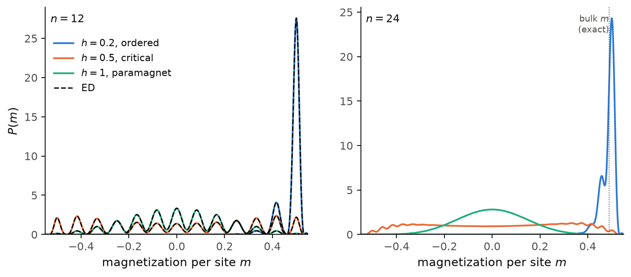
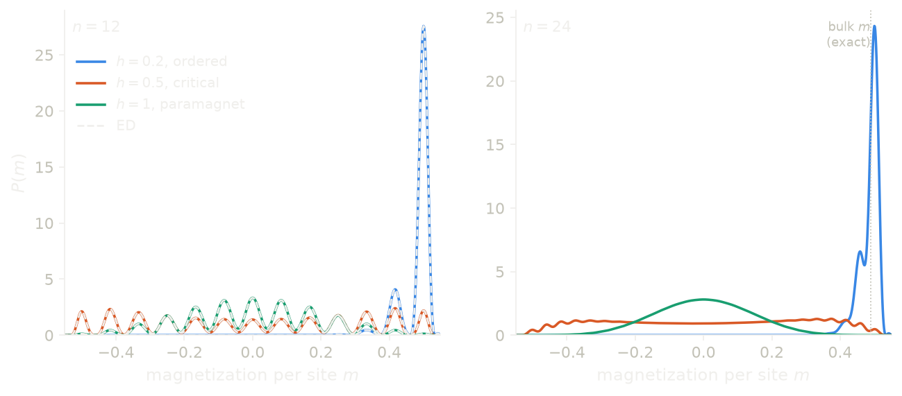
The figure shows \(P(m)\) for the magnetization per site
\(m=\frac1n\sum_iS^z_i\) in the transverse-field Ising chain
\(H=-\sum_iS^z_iS^z_{i+1}-h\sum_iS^x_i\), which is critical at \(h=1/2\).
A small field \(10^{-4}\sum_iS^z_i\) selects one of the two ordered states.
In the ordered phase (\(h=0.2\)), \(P(m)\) is one sharp peak close to the
exact bulk value \(m=0.489\). At the critical field it is broad and flat,
and in the paramagnet (\(h=1\)) it is one peak at \(m=0\). On the left, with
\(n=12\), the DMRG curves lie on the ED curves (dashed lines). There the
peaks are separated, because \(m\) only takes the values \(k/n\). On the
right, with \(n=24\), these values are closer than the resolution set by
delta, so the distribution looks smooth.
Code of this figure (docs/figures/correlators_distribution/)
# Distribution P(m) of the magnetization per site m in the ground state of the
# transverse-field Ising chain H = -sum SzSz - h sum Sx - hz sum Sz, critical
# at h=1/2, from a Chebyshev (KPM) expansion; ED checks DMRG on the small chain.
import numpy as np
from dmrgpy import spinchain

hs = [0.2, 0.5, 1.0]
hz = 1e-4  # tiny longitudinal field that picks one of the two ordered states
n_small, n_large = 12, 24
scale, npol = 0.625, 96  # m in [-1/2,1/2] maps to [-0.8,0.8], 96 moments
# The same npol moments on both solvers: DMRG keeps int(3*scale/delta)+2 and
# ED 4*int(scale/delta), and half a moment more survives the int() rounding.
delta = 3*scale/(npol - 2 + 0.5)
delta_ed = scale/(npol/4 + 0.5)


def chain(n, h):
    """The chain and its magnetization per site m."""
    sc = spinchain.Spin_Chain(["S=1/2"]*n)
    sc.set_hamiltonian(-sum(sc.Sz[i]*sc.Sz[i+1] for i in range(n-1))
                       - h*sum(sc.Sx[i] for i in range(n))
                       - hz*sum(sc.Sz[i] for i in range(n)))
    sc.maxm, sc.kpmmaxm, sc.nsweeps = 60, 60, 12
    return sc, sum(sc.Sz[i] for i in range(n))*(1.0/n)


p_small, p_small_ed, p_large = [], [], []
for h in hs:
    sc, m = chain(n_small, h)
    m_small, p = sc.get_distribution(X=m, delta=delta, scale=scale)
    p_ed = sc.get_distribution(X=m, delta=delta_ed, scale=scale, xs=m_small,
                               mode="ED")[1]
    p_small.append(p.real)
    p_small_ed.append(p_ed.real)
    sc, m = chain(n_large, h)
    m_large, p = sc.get_distribution(X=m, delta=delta, scale=scale)
    p_large.append(p.real)

np.savez("data.npz", h=hs, n_small=n_small, n_large=n_large, m_small=m_small,
         p_small=p_small, p_small_ed=p_small_ed, m_large=m_large,
         p_large=p_large)
import numpy as np
import style

d = np.load("data.npz")
h = d["h"]
names = {0.2: "ordered", 0.5: "critical", 1.0: "paramagnet"}
# bulk magnetization per site of the ordered phase (Pfeuty), m = (1-(2h)^2)^(1/8)/2
m_pfeuty = 0.5*(1-(2*h[0])**2)**0.125


def draw(theme):
    c = style.colors(theme)
    fig, (a, b) = style.figure(2)
    for k, hk in enumerate(h):
        lab = r"$h=%g$, %s" % (hk, names.get(float(hk), ""))
        a.plot(d["m_small"], d["p_small"][k], color=c["series"][k], label=lab)
        b.plot(d["m_large"], d["p_large"][k], color=c["series"][k], label=lab)
    for k in range(len(h)):
        a.plot(d["m_small"], d["p_small_ed"][k], **style.reference(theme),
               label="ED" if k == 0 else None)
    b.axvline(m_pfeuty, color=c["ink2"], lw=0.8, ls=":")
    b.text(m_pfeuty, b.get_ylim()[1]*0.97, " bulk $m$\n (exact)",
           color=c["ink2"], ha="right", va="top", fontsize=8)
    for ax, n in ((a, d["n_small"]), (b, d["n_large"])):
        ax.set_xlabel(r"magnetization per site $m$")
        ax.set_xlim(-0.55, 0.55)
        ax.set_ylim(bottom=0)
        ax.text(0.02, 0.97, r"$n=%d$" % n, transform=ax.transAxes,
                ha="left", va="top")
    a.set_ylabel(r"$P(m)$")
    a.legend(loc="upper left", bbox_to_anchor=(0.0, 0.9))
    return fig


style.main(draw, "correlators_distribution")
The many-body density of states, \(\rho(E)=\sum_n\delta(E-E_n)\), is not a
distribution of this kind: get_distribution computes a ground-state
expectation value, not a trace over all the states, and there is no
method for \(\rho(E)\). For a small chain the full ED spectrum from
get_excited(mode="ED", n=...) (Excited states)
gives it directly.