STM and Kondo spectra
On this page we compute the differential conductance \(dI/dV\) measured by an STM tip above a magnetic atom or a spin chain on a surface. The electrons tunnel from the tip to the sample, and on the way they exchange spin and energy with the spins. We follow the perturbation theory of Ternes, New J. Phys. 17, 063016 (2015), arXiv:1505.04430, to third order in the coupling. The tip couples to one site of the chain. Here the chain is a single spin-1/2 in a magnetic field, with \(H\) in eV:
import numpy as np
from dmrgpy import spinchain
muB, g, B = 5.7883818066e-5, 2.0, 10.0    # eV/T, g-factor, field in T
sc = spinchain.Spin_Chain(["S=1/2"])
sc.set_hamiltonian(g*muB*B*sc.Sz[0])
eV = np.linspace(-4e-3, 4e-3, 161)        # bias in eV
eV, dIdV = sc.get_kondo_spectrum(eV, site=0, Jrho_s=-0.05, U=0.25, T=1.0)
Second order
Second order (order=2) is the Fermi golden rule for spin-flip and
elastic tunneling,
summed over both tunneling directions. Here \(p_i\) is the Boltzmann weight of eigenstate \(i\), \(\epsilon_{if}=E_f-E_i\), and \(\Theta\) a step broadened by temperature. Each excitation of the spins gives a step in \(dI/dV\) at \(eV=\pm\epsilon_{if}\). This is inelastic tunneling spectroscopy (IETS), and the step positions measure the spin excitation energies, for example the Zeeman energy.
Third order
Third order (order=3, the default) adds two terms. Both sum over
every eigenstate \(m\) as a virtual intermediate state. The Kondo term
involves three spin matrix elements and a logarithmic function
\(F(\epsilon,T)\). It gives a peak at zero bias, which splits into two
peaks at the Zeeman steps in a field. The potential-interference term,
present when U is not zero, makes the spectrum asymmetric in bias. The
second-order and Kondo terms are even in \(eV\), and the potential term is
odd in \(eV\).
At the parameters of the paper (\(S=1/2\), \(B=0\), \(T=1\) K, \(J\rho_s=-0.05\), \(\omega_0=20\) meV), the zero-bias peak divided by \(2\pi\) is 1.13 for \(U=0\) and 1.39 for \(U=0.25\), as in the paper's figures. In a field the code departs from the paper in one place: the exchange diagram of the Kondo term has its logarithm at \(F(eV-(\epsilon_f-\epsilon_m))\), which is what an exact second-order T-matrix gives, and not at the argument of the paper's eq. 25. The two agree at zero field for \(S=1/2\) and at zero bias. In the cases tested with a field or anisotropy, they differ by 5 to 20 per cent of the third-order term. The keywords are:
site: the site under the tip.Jrho_s: the dimensionless Kondo coupling \(J\rho_s\), in the sign convention of the paper (which uses \(-0.05\)).U: the ratio of potential scattering to spin scattering.T: the temperature in kelvin.kB(default in eV/K) converts it to the energy unit of \(H\).omega0,Gamma0: the band cutoff and the lifetime broadening of the Kondo function \(F\).T0: the tunneling strength. It only sets the overall scale.order: 2, 3, or"LL"(see Leading logs).
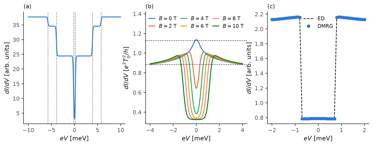
Left: the second-order spectrum of an \(S=2\) atom with
\(H=D(S^z)^2+E[(S^x)^2-(S^y)^2]\), \(D=-1.55\) meV and \(E=0.31\) meV (Fe on
Cu\(_2\)N), at \(T=0.5\) K. The steps sit at the excitation energies of the
spin multiplet, 0.18, 3.90 and 5.76 meV (dotted lines), which come from
the exact \(5\times5\) Hamiltonian. Middle: the third-order spectrum of an
\(S=1/2\) with \(J\rho_s=-0.05\), \(U=0\) and \(T=1\) K, divided by \(2\pi\)
to give units of \(e^2T_0^2/h\). At \(B=0\) there is a Kondo peak at zero bias. Its height,
1.137, and its value at \(\pm4\) mV, 0.885, match the paper's 1.13 and 0.886
(dotted lines). In a field the peak splits. The spectrum drops in the gap
\(|eV|<g\mu_BB\), and the Kondo term gives two peaks just outside the
Zeeman steps. Right: the \(T=0\) spectrum of a 3-site chain
from mode="DMRG" agrees with mode="ED" to 0.5 per cent (see
ED and DMRG).
Code of this figure (docs/figures/kondo_dIdV/)
# STM dI/dV of magnetic atoms and chains, in the third-order perturbation
# theory of Ternes (NJP 17, 063016). Energies in eV, temperatures in kelvin.
import numpy as np
from dmrgpy import spinchain

muB = 5.7883818066e-5  # eV/T

# (a) inelastic steps of an S=2 atom, D Sz^2 + E (Sx^2 - Sy^2) (Fe on Cu2N)
D, E = -1.55e-3, 0.31e-3
sc = spinchain.Spin_Chain(["S=2"])
sc.set_hamiltonian(D*sc.Sz[0]*sc.Sz[0] + E*(sc.Sx[0]*sc.Sx[0] - sc.Sy[0]*sc.Sy[0]))
eV_a, dIdV_a = sc.get_kondo_spectrum(np.linspace(-10e-3, 10e-3, 401), site=0,
                                     order=2, T=0.5)
# reference: excitations of the exact 5x5 Hamiltonian that S+, S-, Sz reach
m = np.arange(2.0, -3.0, -1.0)
sz, sp = np.diag(m), np.diag(np.sqrt(6 - m[1:]*(m[1:] + 1)), 1)
sx, sy = (sp + sp.T)/2, (sp - sp.T)/2j
w, v = np.linalg.eigh((D*sz @ sz + E*(sx @ sx - sy @ sy)).real)
weight = sum(f*np.abs(v.T @ op @ v[:, 0])**2
             for f, op in ((0.5, sp), (0.5, sp.T), (1.0, sz)))
eps_a = (w - w[0])[1:][weight[1:] > 1e-8]

# (b) Kondo peak of an S=1/2 in a field B (in tesla), in units of e^2 T0^2/h
B_b = [0.0, 2.0, 4.0, 6.0, 8.0, 10.0]
eV_b = np.linspace(-4e-3, 4e-3, 161)
dIdV_b = []
for B in B_b:
    sc = spinchain.Spin_Chain(["S=1/2"])
    sc.set_hamiltonian(2.0*muB*B*sc.Sz[0])
    _, y = sc.get_kondo_spectrum(eV_b, site=0, Jrho_s=-0.05, U=0.0, T=1.0,
                                 order=3, omega0=20e-3)
    dIdV_b.append(y/(2*np.pi))

# (c) 3-site Heisenberg chain with a field on the first site, at T=0:
# DMRG (KPM and a two-time TDVP construction) against ED
sc = spinchain.Spin_Chain(["S=1/2"]*3)
sc.maxm, sc.nsweeps = 30, 15
sc.set_hamiltonian(2.0*muB*10.0*sc.Sz[0]
                   + sum(0.01*(sc.Sx[i]*sc.Sx[i+1] + sc.Sy[i]*sc.Sy[i+1]
                               + sc.Sz[i]*sc.Sz[i+1]) for i in range(2)))
sc.get_gs()
eV_c = np.linspace(-2e-3, 2e-3, 41)
kw = dict(site=0, Jrho_s=0.05, U=0.0, T=0.0, order=3, omega0=2e-3, Gamma0=2e-3)
_, dIdV_ed = sc.get_kondo_spectrum(eV_c, mode="ED", **kw)
_, dIdV_dmrg = sc.get_kondo_spectrum(
    eV_c, mode="DMRG", submode="KPM", delta=2e-5,
    es=np.linspace(-3e-3, 3e-3, 800), dt2=150.0, n_t2_half=20, dtau=150.0,
    n_tau_half=20, **kw)

np.savez("data.npz", eV_a=eV_a, dIdV_a=dIdV_a, eps_a=eps_a, B_b=B_b, eV_b=eV_b,
         dIdV_b=dIdV_b, eV_c=eV_c, dIdV_ed=dIdV_ed, dIdV_dmrg=dIdV_dmrg)
import numpy as np
import style

d = np.load("data.npz")
mev = 1e3


def draw(theme):
    c = style.colors(theme)
    fig, (ax1, ax2, ax3) = style.figure(3)
    for ax, t in zip((ax1, ax2, ax3), "abc"):
        ax.text(0.0, 1.02, "(%s)" % t, transform=ax.transAxes, va="bottom",
                color=c["ink"])

    for e in d["eps_a"]:  # exact step positions
        for s in (+1, -1):
            ax1.axvline(s*e*mev, color=c["ink2"], ls=":", lw=style.LW_REF)
    ax1.plot(d["eV_a"]*mev, d["dIdV_a"], color=c["series"][0], lw=style.LW)
    ax1.set_xlabel(r"$eV$ [meV]")
    ax1.set_ylabel(r"$dI/dV$ [arb. units]")

    for j, B in enumerate(d["B_b"]):
        ax2.plot(d["eV_b"]*mev, d["dIdV_b"][j], color=c["series"][j],
                 lw=style.LW, label=r"$B=%g$ T" % B)
    for v in (1.13, 0.886):  # Ternes at B=0: zero bias and +-4 mV
        ax2.axhline(v, color=c["ink"], ls=":", lw=style.LW_REF)
    ax2.set_xlabel(r"$eV$ [meV]")
    ax2.set_ylabel(r"$dI/dV$ [$e^2T_0^2/h$]")
    ax2.legend(ncol=3, loc="upper center", handlelength=1.2, columnspacing=0.8)
    ax2.set_ylim(0.28, 1.42)

    ax3.plot(d["eV_c"]*mev, d["dIdV_ed"], **style.reference(theme), label="ED")
    ax3.plot(d["eV_c"]*mev, d["dIdV_dmrg"], "o", color=c["series"][0],
             ms=style.MS, label="DMRG")
    ax3.set_xlabel(r"$eV$ [meV]")
    ax3.set_ylabel(r"$dI/dV$ [arb. units]")
    ax3.legend()
    return fig


style.main(draw, "kondo_dIdV")
Leading logs
We will now see how to go beyond third order. Each further order adds one
more power of the same logarithm, \(J\rho_s\ln(\omega_0/|eV-\epsilon|)\).
Near zero bias and near the steps this number is not small, and the third
order fails there. order="LL" sums these leading logarithms to all
orders with the perturbative renormalization group. The couplings run as
the band cutoff is lowered, and each logarithm stops at the energy of its
own virtual process, so in a field or with anisotropy the couplings depend
on the energy of the electron (Rosch, Paaske, Kroha, Wölfle,
cond-mat/0408506; Rosch, Costi, Paaske, Wölfle, cond-mat/0301106). The
renormalized tip vertex then goes into the second-order formula. To first
order in \(J\rho_s\) this is exactly order=3. At \(T>0\) the cutoff of each
logarithm is averaged over the thermal window of the electrodes, with the
same weight as the third order, so the first order is order=3 at the same
temperature, and the excited states of the sample are occupied as in
mode="ED". At \(T>0\) the memory grows with the number of occupied
states, and mem_gb=4 cuts the biases in groups so that each flow stays
below about 4 GB. When \(H\) conserves \(S^z\) (no field, or a field along
\(z\)) the flow at \(T=0\) uses this symmetry on its own from 32 states on,
with the same result; sz_blocks=False turns this off.
sc = spinchain.Spin_Chain(["S=1/2"])
sc.set_hamiltonian(0*sc.Sz[0])
eV = np.linspace(-4e-3, 4e-3, 161) + 1e-5
eV, dIdV = sc.get_kondo_spectrum(eV, Jrho_s=-0.05, U=0.0, T=0.0, order="LL")
At the coupling of the paper the zero-bias peak is higher than at third
order: \(dI/dV/2\pi\) is 1.95 at \(eV=10\) \(\mu\)eV against 1.31, and 1.06 at
1 meV against 0.98. Far from zero bias the two agree, 0.92 against 0.88 at
4 meV. The method is still perturbative. It fails at the Kondo temperature,
where the running coupling reaches order one, and there it returns NaN
with a warning (for example at \(J\rho_s=-0.2\) near zero bias). It also
warns when the running coupling passes 0.5, which can happen near a step
while the zero-bias coupling is still small. It
renormalizes the couplings and not the energies, so the steps stay at the
bare excitation energies. The derivation and its checks are in
docs/new_methods/kondo_leading_log/ in the repository.
Backends
order="LL" works with mode="ED" only, at any temperature. It runs
on a GPU, with the same numbers, when the array backend is JAX:
from dmrgpy.pyitensor import backend and backend.set_backend("jax")
before the call. The memory grows as the square of the number of
states, so a large impurity needs a card with much memory and full
double precision: 13 spins 1/2 take about 110 GB. JAX gives a process
only 75% of the card by default, so for such a run set
XLA_PYTHON_CLIENT_MEM_FRACTION=0.95 in the environment before
Python starts. Above 2000 states
the full diagonalization is refused unless
dmrgpy.algebra.algebra.maxsize is raised first.
ED and DMRG
mode="ED" (the default) diagonalizes the full
Hamiltonian, since every eigenstate enters as a virtual state. It works
at any temperature, on small chains. mode="DMRG"
works at \(T=0\) and never needs excited states (submode="TASK" below also
takes the temperature of the electrodes). The second-order and
potential terms come from the dynamical correlator, and the
Kondo term from a real-time evolution of a three-point function. It runs
on itensor_version=3, "python" and "julia_live", on chains of at
least 3 sites.
Here the chain has 3 sites, with the field on the first one and a weak
Heisenberg coupling. Without a field the ground state is degenerate, see
n_gs below:
sc = spinchain.Spin_Chain(["S=1/2"]*3)
h = g*muB*B*sc.Sz[0]
for i in range(2):
    h = h + 0.01*(sc.Sx[i]*sc.Sx[i+1] + sc.Sy[i]*sc.Sy[i+1] + sc.Sz[i]*sc.Sz[i+1])
sc.set_hamiltonian(h)
eV = np.linspace(-2e-3, 2e-3, 41)
es = np.linspace(-3e-3, 3e-3, 800)
eV, dIdV = sc.get_kondo_spectrum(eV, Jrho_s=-0.05, U=0.0, T=0.0, order=3,
               omega0=2e-3, Gamma0=2e-3, mode="DMRG", submode="KPM",
               delta=2e-5, es=es,
               dt2=150.0, n_t2_half=20, dtau=150.0, n_tau_half=20)
These keywords have no default and must be chosen for the problem:
es: the frequency grid of the dynamical correlator. Fororder=2it must cover the transitions below \(\max|eV|\). WithUnot zero it must cover the whole spin excitation spectrum of the site, plus a fewdelta. The grid may be non-uniform. The grid must start severaldeltabelow 0 (the elastic line at zero energy is cut otherwise) and pass \(\max|eV|\), and a warning says when it does not.delta,submode: the broadening and the method of the dynamical correlator.dt2,n_t2_half,dtau,n_tau_half: the two time grids of the Kondo term. They must resolve the time scales \(1/\omega_0\) and \(1/\Gamma_0\), so the default \(\omega_0\) and \(\Gamma_0\) need very long grids. Too coarse a grid gives a wrong result without any error, so compare withmode="ED"on a small chain first.n_gs: the number of degenerate ground states. With a degenerate ground state,mode="ED"averages over the multiplet, while DMRG returns one member.n_gs=gmakes DMRG average overgstates too.
With submode="TASK", the default on itensor_version=3, "python"
and "julia_live", there is no frequency or time grid at all. On
itensor_version=2 the default stays "KPM" with the two-time route
above. The tangent-space Krylov method of
Choosing a correlator method gives the ground
state and the excited states that the spin of the site reaches, as
discrete energies, and the exact sums of mode="ED" run over them:
eV, dIdV = sc.get_kondo_spectrum(eV, Jrho_s=-0.05, U=0.0, T=0.0, order=3,
               omega0=2e-3, Gamma0=2e-3, mode="DMRG", submode="TASK",
               nkry=100)
The result is exact when maxm holds the whole Hilbert space (with
sc.cutoff = 0) and nkry is large enough; with a smaller maxm the
excited states are one-site changes of the ground state, which moves the
steps slightly. It takes only nkry (default 100, increase until the
spectrum stops changing) and n_gs.
At \(T=0\) every excited state is a sharp step of \(dI/dV\). On a long chain
the Krylov space resolves only the lowest excited states one by one, and
the others are steps at energies that still move with nkry. A warning
says how many, and how large the largest of these steps is. A larger
nkry makes them fewer. On a long chain some always remain, so compare
such curves only at a bias resolution above the spacing of the steps.
With T>0 the steps and the Kondo peak are broadened by the temperature
of the tip and of the substrate, as in an experiment, and the sample stays
in its ground state:
eV, dIdV = sc.get_kondo_spectrum(eV, Jrho_s=-0.05, U=0.0, T=0.5, order=3,
               omega0=2e-3, Gamma0=2e-3, mode="DMRG", submode="TASK",
               nkry=100)
This is the thermal spectrum as long as \(k_BT\) is well below the lowest
excitation of the sample. The call raises an error when the Boltzmann
factor of the lowest excitation that the spin of the site reaches is
above \(10^{-3}\); use mode="ED" then. An excitation that this spin does
not reach is not checked. A degenerate ground state needs n_gs, as at
\(T=0\). Once the thermal width \(5.4\,k_BT\) is larger than the spacing of
the steps, the curve no longer depends on the steps that are not
converged, and a smaller nkry is enough, as long as the lowest
excitation itself is converged.
See examples/kondo/kondo_third_order_dmrg_VS_ED, which is the right
panel of the figure in Third order, and
examples/kondo/kondo_third_order_task_VS_ED. The tip couples to one
site only; several sites with independent couplings are not implemented.
Larger clusters at finite temperature
mode="ED" diagonalizes the whole Hamiltonian, so it stops at about 10
spins 1/2. At a temperature \(T\) only the states within a few \(k_BT\) of the
ground state are occupied. An occupied state \(i\) reaches, through the spin
of the tip site, only the states in the span of \(S_a|i\rangle\) and of \(H\)
applied to them. submode="KRYLOV" uses both facts. It finds the occupied
states with a sparse eigensolver. For each one it builds a single Krylov
space started from \(S_x|i\rangle\), \(S_y|i\rangle\) and \(S_z|i\rangle\)
together, and it runs the sums of mode="ED" over the states of that
space. It works with any Hamiltonian, also when \(S_z\) is not conserved,
for example in a field that turns from site to site:
n = 8
sc = spinchain.Spin_Chain(["S=1/2"]*n)
h = 0
for i in range(n-1):
    h = h + 1e-3*(sc.Sx[i]*sc.Sx[i+1] + sc.Sy[i]*sc.Sy[i+1] + sc.Sz[i]*sc.Sz[i+1])
for i in range(n):
    h = h + 2e-4*(np.cos(2*np.pi*i/3)*sc.Sx[i] + np.sin(2*np.pi*i/3)*sc.Sz[i])
sc.set_hamiltonian(h)
eV = np.linspace(-4e-3, 4e-3, 101) + 1e-5
eV, dIdV = sc.get_kondo_spectrum(eV, site=1, Jrho_s=-0.05, U=0.2, T=1.0,
               submode="KRYLOV", nkry=100)
The result is the one of mode="ED" once every Krylov space holds all
the states that the spin reaches, apart from the occupied states that are
dropped. On this chain the two differ by about \(10^{-8}\) of the peak at 1 K.
nkry: each Krylov space holds at most3*nkrystates (default 100). Increase it until the spectrum stops changing.p_cut: occupied states whose Boltzmann weight is belowp_cuttimes that of the ground state are dropped (default \(10^{-8}\)), and \(dI/dV\) changes by about that much.su2: when \(H\) conserves the total spin, the default (None) takes one member of each spin multiplet with the weight \(2S+1\), which needs fewer occupied states, and otherwise every state.Trueraises when \(H\) does not conserve the total spin, andFalsealways takes every state.tol: with a value such as \(10^{-8}\), a Krylov space stops before3*nkrystates once every state that can be a final state (up to \(\max\lvert eV\rvert\) above the initial state, plus \(40k_BT\)) is converged totoltimes the scale of \(H\). Useful with a largenkryand a narrow bias window. The default (None) never stops early.
The route is third order. order="LL" needs every eigenstate and raises
with submode="KRYLOV". See examples/kondo/kondo_krylov_thermal_VS_ED.
Hubbard chains
The same method works on the spinful fermion chains,
Spinful_Fermionic_Chain and Spinful_Fermionic_Chain_Native. The tip
then couples to the electron spin of the site,
\(\mathbf{S}_i=\frac12 c^\dagger_i\boldsymbol{\sigma}c_i\). The spectrum
includes the charge fluctuations that a spin model leaves out. At half
filling and large \(U\) the Hubbard chain maps onto a Heisenberg chain with
\(J=4t^2/U\), so the two spectra can be compared with the bias in units of
\(J\):
import numpy as np
from dmrgpy import fermionchain
n, t, U = 6, 1.0, 16.0
J = 4*t**2/U
fc = fermionchain.Spinful_Fermionic_Chain_Native(n)
h = 0
for i in range(n-1):
    h = h - t*(fc.Cdagup[i]*fc.Cup[i+1] + fc.Cdagdn[i]*fc.Cdn[i+1])
h = h + h.get_dagger()
for i in range(n):
    h = h + U*(fc.Nup[i]-0.5)*(fc.Ndn[i]-0.5)
fc.set_hamiltonian(h)
fc.set_conserved_sector(Nf=n)       # half filling, for mode="ED"
eV, dIdV = fc.get_kondo_spectrum(np.linspace(-3*J, 3*J, 240), Jrho_s=-0.05,
               T=0.0, kB=1.0, omega0=10*J, Gamma0=1e-2*J)
With mode="ED" a sector of fixed electron number Nf is exact at
\(T=0\), since \(\mathbf{S}_i\) does not change the number of electrons. At
\(T>0\) it gives the canonical ensemble at that Nf. A sector of fixed
Sz raises, since \(S_\pm\) leaves it. mode="DMRG" with
submode="TASK" works on both classes. Use
Spinful_Fermionic_Chain_Native: there the site is one tensor, while on
Spinful_Fermionic_Chain the spin of the site acts on two tensors, so a
truncated maxm was less accurate in our tests. As \(U/t\) grows the Hubbard spectrum
approaches the Heisenberg one. The difference falls as \((t/U)^2\) once
\(U/t\) is a few tens; below that, higher orders in \(t/U\) still matter. The
weight of the steps drops with the double occupancy, and the steps move
with the corrections to \(J\). See
examples/kondo/kondo_third_order_hubbard_VS_heisenberg.
Orbital-resolved IETS of a magnetic atom
dmrgpy.atom describes a single atom with five \(d\) orbitals instead of a
chain. generate_atom builds a Spinful_Fermionic_Chain whose sites are
the orbitals, with a crystal field tij, spin-orbit coupling soc, the
interactions U and J, a magnetic field B acting as
\(2\mathbf S+\mathbf L\), and Ne electrons. Two IETS signals are
available:
from dmrgpy import atom
orbs = ["dxy", "dyz", "dz2", "dxz", "dx2y2"]
tij = np.diag([0.0, 0.05, 0.6, 0.05, 0.6])           # crystal field, eV
fc = atom.generate_atom(orbs=orbs, tij=tij, Ne=2, soc=0.03, U=4., J=0.5)
es = np.linspace(0., 0.1, 301)
x, y = atom.get_spinflip(fc, es=es, iorb=2, delta=1e-3)
x, y = atom.get_orbital_cotunneling(fc, es=es, iorb=2, delta=1e-3)
get_spinflip: the spin-flip signal, \(\sum_aS_{aa}(\omega)\) built from \(S^a-\langle S^a\rangle\) on orbitaliorb.get_orbital_cotunneling: the orbital cotunneling signal, from \(c^\dagger_{\texttt{iorb}\,\sigma}c_{j\sigma'}\) summed over the other orbitals \(j\) and both spins.
iorb is the orbital the tip couples to, for example \(d_{z^2}\) for a tip
on top of the atom. With a crystal field, different orbitals give
different weights and different peak positions. Both functions use ED.
The low multiplet of an atom is often nearly degenerate, so the remarks
of Degenerate ground states on dex and T apply here. See
examples/kondo/atom_iets_orbital_resolved.
Kondo screening on a Wilson chain
We now ask a different question: is the spin of an impurity screened by the conduction electrons, and by which electrons? We follow the NRG-MPS method of Stocker and Zilberberg, arXiv:2501.10746. The Anderson impurity
is coupled to a Wilson chain: the band on \([-D,D]\) is cut at the energies \(\pm D\Lambda^{-m}\), and the Lanczos tridiagonalization of the levels gives the hoppings \(t_n \sim \Lambda^{-n/2}\). Site \(n\) resolves the energy \(D\Lambda^{-n/2}\), so the chain must be long enough to reach below the Kondo temperature \(T_K\). DMRG gives the ground state, and from it we compute
\(M_{\text{imp}}\) is the probability that the impurity is singly occupied, and \(M_n\) says where the screening cloud sits along the chain. A screened moment has \(M_{\text{imp}}\) close to 1 and \(M_{\text{env}} = -M_{\text{imp}}\). We also project the ground state on a singly occupied impurity and take its Schmidt coefficients between impurity and bath: two equal values \(1/\sqrt2\) for the Kondo singlet, one value 1 for a free, polarized moment.
from dmrgpy import wilsonchain
fc = wilsonchain.anderson_chain(13, ed=-0.5, U=1.0, tD=0.3, Lambda=3.0, B=0.0)
fc.maxm = 100
fc.nsweeps = 12
r = fc.get_kondo_screening()
print(r["M_imp"], r["M_env"], r["M_n"], r["schmidt"])
The bandwidth is \(D=U\) and the density of states is flat and normalized,
so \(\Gamma = \pi t_D^2/(2D)\), and here \(T_K \approx 0.017\,U\). The result
is \(M_{\text{imp}} = 0.83\), \(M_{\text{env}} = -0.83\) and Schmidt
coefficients \((0.707, 0.707)\): a Kondo singlet. In zero field
\(M_{\text{env}} = -M_{\text{imp}}\) holds exactly for any singlet, so the
information is in \(M_{\text{imp}}\), in the profile \(M_n\), and in the
response to a field. With B the larger Schmidt coefficient goes from
\(1/\sqrt2\) to 1 when \(B\) passes \(T_K\). The field also polarizes the bath,
and \(M_n\) is not a connected correlator, so in a strong field
\(M_{\text{env}}\) turns positive.
With two levels, ed and tD are lists of two. Each level couples to its
own Wilson chain, and \(U\) acts between all four spin-orbitals, so at
\(\epsilon_d=-U/2\) the impurity holds one electron. Then M_imp and
M_n are given per level, M_env[l][k] is the screening of level l by
chain k, and there are four Schmidt coefficients. Equal couplings give
an SU(4) Kondo singlet, with four values \(1/2\). Unequal couplings split
them in two pairs, and the splitting grows with the chain length, toward
the SU(2) singlet of the level with the larger coupling.
The Kondo cloud along a real-space lead
How far from the impurity does the screening happen? A Wilson chain does not say it, since its sites are energy shells and not positions. We follow Holzner, McCulloch, Schollwöck, von Delft and Heidrich-Meisner, PRB 80, 205114 (2009), and put the dot at the end of a plain tight-binding lead of \(L-1\) sites, \(L\) sites in total:
The cloud is read from the integrated spin correlation
meaning that \(1-\Sigma(x)\) is the part of the impurity spin screened by the first \(x\) lead sites. In a total-spin singlet \(\langle \vec S_{\text{tot}}^2\rangle=0\) gives \(\sum_i \langle \vec S_d\cdot\vec S_i\rangle = -\langle \vec S_d^2\rangle\), so \(\Sigma(L-1)=0\) exactly. This needs \(L\) even at half filling; with \(L\) odd the ground state is a doublet. The screening length is the distance where a fraction \(a\) of the spin is screened, \(\xi_a(L) = \min\{x : \Sigma(x) \le 1-a\}\), with \(a=0.9\) as the reference. It grows with \(L\) and saturates once the lead is longer than the cloud. The scale to compare with is \(\xi_K^0 = \hbar v_F/T_K\), with \(v_F=2t\) and
The paper finds \(\xi_{0.9} \approx 6.7\,t/T_K\) for \(U/\Gamma \gtrsim 2\).
from dmrgpy import kondocloud
fc = kondocloud.anderson_lead(40, ed=-0.5, U=1.0, Gamma=0.5)
fc.maxm = 80
fc.nsweeps = 12
fc.cutoff = 1e-10
r = fc.get_kondo_cloud(a=[0.75, 0.9])
print(r["Sigma"], r["xi"], r["sum_rule"])
print(6.7/kondocloud.kondo_temperature(1.0, 0.5))
Here \(U/\Gamma=2\) and \(T_K=0.32\). The result is \(\xi_{0.75}=5\) and \(\xi_{0.9}=15\), the same at \(L=60\), and \(\Sigma(L-1)=4\times10^{-6}\), the truncation error. \(\Sigma(x)\) drops in steps of two sites: the odd sites screen and the even sites add almost nothing, the even-odd effect of a half-filled lead, so \(\xi_a\) comes out odd. At \(U/\Gamma=3\) we get \(\xi_{0.75}=9\), again the same at \(L=40\) and \(60\), so \(\xi_{0.75}T_K\) is 1.61 and 1.60 for the two couplings, meaning that the cloud scales as \(1/T_K\). The paper's own numbers give 1.8. For \(\xi_{0.9}\) at \(U/\Gamma=2\) we get \(4.8/T_K\); \(U/\Gamma=2\) is at the edge of the Kondo regime, where the paper also sees deviations from \(6.7/T_K\). At \(U/\Gamma=3\) and 4, \(\xi_{0.9}\) still grows from \(L=40\) to \(L=60\): the cloud does not fit in the lead yet.
L: the total number of sites, dot included. Take it even.Gamma,U,ed: the hybridization, the repulsion and the level, in units oft. The cloud grows as \(1/T_K\), so it fits only for small \(U/\Gamma\): on leads of 40 to 60 sites \(\xi_{0.75}\) saturates up to \(U/\Gamma=3\).half_filling=True: fixes \(N=L\) electrons, as the paper does. It is needed away from \(\epsilon_d=-U/2\), where particle-hole symmetry no longer fixes the filling. Onitensor_version="python"this sector converged here for leads up to 30 sites, not at 40.Bandconnected=True: a field on the dot. Then \(S^z_{\text{tot}}\) is the only conserved spin, and we use the connected form \((\langle S^z_d S^z_i\rangle - \langle S^z_d\rangle\langle S^z_i\rangle)/ (\langle S^z_d S^z_d\rangle - \langle S^z_d\rangle^2)\), which has no sum rule.r["mu"]is the moment \(\langle (S^z_d)^2\rangle - \langle S^z_d\rangle^2\).maxm: a metallic lead is entangled at every bond, so it needs a large bond dimension. At \(L=40\),maxm=64gave \(\xi_{0.9}=14\) andmaxm=80and 100 gave 15. A too small bond dimension also breaks the singlet, and then \(\Sigma(L-1)\) is not 0; a warning says so abovesum_rule_tol.
The scaling collapses of the paper, \(\Sigma\) against \(x/\xi_K\) and
\(\xi_a(L)/\xi_a\) against \(L/\xi_a\), are fits on these numbers. See
examples/kondo/kondo_cloud_real_space.
The Wilson chain keywords
n: the number of Wilson chain sites per level. It sets the lowest energy, \(D\Lambda^{-n/2}\), which must be below \(T_K\). Take \(n\) odd: with \(n\) even the ground state has an odd number of electrons, so it is degenerate and not a singlet, and one member of it looks unscreened.Lambda: the discretization. A larger value reaches low energies with fewer sites, at the price of a coarser band.B: a field \(B S^z\) on the impurity, and a rigid shift \(\pm B\) of the bath bands.dos: a function giving the shape of the density of states, flat if not given.maxm: the Wilson chain ground state needs a bond dimension of 100 or more. Too small amaxmgives a state that breaks spin symmetry, which looks like an unscreened moment: \(M_{\text{env}} \neq -M_{\text{imp}}\) and unequal Schmidt coefficients in zero field. Check against a largermaxm.
The diagnostics are expectation values, so mode="ED" gives the exact
values on a short chain, and get_kondo_screening(imp=..., bath=...)
works on any spinful chain. See examples/kondo/kondo_screening_field and
examples/kondo/kondo_screening_su4.
Open Wilson chains
We now see how to keep the bath modes that a Wilson chain drops. We follow Bruognolo et al., arXiv:1611.05291. A chain of \(N\) sites stands for the bath at the temperature \(T \sim \Lambda^{-N}\), and the modes below that scale are missing. They do not only broaden the levels, they also shift them, because the bath correlator at zero frequency,
is not zero when the spectrum \(A(\omega)\) is not symmetric. For a bosonic bath it is never symmetric. A chain that misses part of this shift gives a renormalized impurity energy that depends on \(N\), so on \(T\). This is what is called the mass-flow problem.
The open Wilson chain is a continued fraction of the bath correlator. At site \(k\) the self-energy is split by energy: the part inside the window \(\Lambda^{-(k+1)}\) times the band becomes site \(k+1\), the rest stays as the own bath \(F_k\) of site \(k\), with the coupling \(t^F_k\). The chain with all these baths is exact. The renormalized chain keeps only the static part of the baths it drops, as onsite shifts,
Chain C0 has no shifts, C1 the fast shifts only, C2 also the slow shift of the last site. C2 gives \(\mathrm{Re}\, G_{\text{bath}}(0)\) exactly at any length, meaning that a static quantity does not drift with \(N\).
from dmrgpy import wilsonchain
owc = wilsonchain.open_wilson_chain(20, Lambda=2.0, band=(0.0, 1.0),
                                    dos=lambda e: e**0.4)
for kind in ["C0", "C1", "C2"]:
    eps, t = owc.renormalized(10, kind=kind)
    print(kind, wilsonchain.chain_green(eps, t).real)

bc = wilsonchain.spin_boson_chain(6, alpha=0.1, s=0.4, Delta=0.1, eps=0.01,
                                  kind="C2", maxnb=8)
bc.maxm = 40
bc.nsweeps = 20
print(bc.vev(bc.x_imp).real)
For the sub-Ohmic bath \(A \propto \omega^{0.4}\) the exact value is
\(-(s+1)/s = -3.5\). On 10 sites C0 gives \(-2.44\), C1 gives \(-3.42\), and C2
gives \(-3.5\) to 1e-15. The arrays owc.eps, owc.tS, owc.tF, owc.dF
and owc.dS are the chain, and owc.bath_spectrum(k, omega, eta) is the
spectrum \(\Gamma^F_k(\omega)\) of the own bath of site \(k\).
The second part is the spin-boson model,
\(H = -\frac{\Delta}{2}\sigma_x + \frac12\sigma_z\left(\epsilon + t_{\text{imp}}(b+b^\dagger)\right) + H_{\text{bath}}\),
with \(\Gamma(\omega) = 2\alpha\,\omega_c^{1-s}\omega^s\), on a C2 chain of 6
bosonic sites. The spin is site 0, a two-level site, and bc.x_imp is
\(\sigma_z\). Here \(\langle\sigma_z\rangle = -0.90\) already at
\(\epsilon = 0.01\), a strong response of the spin to the bias. Its response to the bias, \(\chi = d\langle\sigma_z\rangle/d\epsilon\)
on a chain of length \(N\), is the susceptibility at \(T \sim \Lambda^{-N}\),
as in the paper. oscillator_chain builds the dissipative harmonic
oscillator in the same way. That model is quadratic, so its
susceptibility \(1/(\Omega - 2\alpha/s)\) is known exactly. The standard
Wilson chain at \(\Lambda=2\), \(\alpha=0.1\), \(s=0.4\), \(\Omega=1\) gives 1.67 on
4 sites and 1.93 on 40 sites instead of 2, while C2 gives 2 at every
length, and DMRG on C2 agrees with it to 1e-5.
n: the number of chain sites. Site \(k\) has the energy \(\Lambda^{-k}\) times the band, on a bosonic and on a fermionic bath.Lambda: the factor by which the slow window shrinks per site.band,dos: the support and the shape of the bath spectrum. A bosonic bath hasband=(0, wc).kind:"C0","C1"or"C2". Use C2 to remove the mass flow.anderson_chain(..., kind="C2")andboson_bath_chaintake it too, and"standard"is the Wilson chain of the section above. Inanderson_chainthe factor per site is \(\Lambda^{1/2}\), sonandLambdamean the same there for every kind.nsub: levels per factor \(\Lambda\) in the fine discretization of the bath. The chain coefficients converge as \(1/\texttt{nsub}\), about 1% at the default 8. The static identities hold at any value.maxnb: bosons per chain site. The C2 shift lowers the energy of the last site, so that site needs more bosons near a critical point.
What we neglect is the dynamics of the dropped baths: only their static
shift is kept, so the chain has no dissipation. For a fermionic band with
a finite density of states at the Fermi level the self-energies have an
imaginary part at \(\omega=0\), and then C2 is an approximation, not an
identity. For a symmetric band all the shifts vanish, and C0, C1 and C2
are the same chain. The finite-temperature NRG averages of the paper are
not used: as in its variational MPS results, the temperature is the length
of the chain. See examples/kondo/open_wilson_chain_mass_flow.
Spin excitations on a superconductor
When the spin is weakly coupled to the superconductor, for instance a molecule whose ligand separates the magnetic ion from the surface, we do not need the Wilson chain. The second-order spectrum of Second order is a golden rule between the eigenstates of the spin alone, and the gap only changes the density of states the electron tunnels into. The current is
with \(C_{st}\) the same with \(f\) and \(1-f\) exchanged, \(\epsilon_{fi} = E_f - E_i\), and \(\rho_t\), \(\rho_s\) the Dynes densities of states of tip and sample, \(\rho(\omega) = \mathrm{Re}\left[(\omega + i\gamma)/\sqrt{(\omega + i\gamma)^2 - \Delta^2}\right]\). For \(\rho = 1\) this is the step \(\Theta(eV - \epsilon_{fi})\) of the normal metal. With a normal tip at \(T=0\), \(dI/dV\) of each transition is \(\rho_s(eV - \epsilon_{fi})\), meaning that every step becomes a coherence peak at \(eV = \Delta_s + \epsilon_{fi}\). With a superconducting tip the peaks move to \(\pm(\Delta_s + \Delta_t + \epsilon_{fi})\), and at \(T > 0\) thermal quasiparticles add peaks at \(\pm|\Delta_s - \Delta_t| \pm \epsilon_{fi}\). This is how a superconducting tip gives inelastic spectroscopy a resolution better than the thermal width.
import numpy as np
from dmrgpy import spinchain
from dmrgpy.ysrtk import bcsperturbative
D, Delta = 0.7e-3, 1.35e-3
sc = spinchain.Spin_Chain(["S=5/2"])
sc.set_hamiltonian(D*sc.Sz[0]*sc.Sz[0])
eV = np.linspace(-6e-3, 6e-3, 2401)
eV, dIdV = bcsperturbative.get_spin_excitation_spectrum(sc, eV, T=1.2,
        U=1.15, Delta_s=Delta, Delta_t=Delta, gamma=1e-2*Delta)
This is the spin 5/2 of Fe-OEP-Cl on Pb measured with a Pb tip by
Heinrich, Braun, Pascual and Franke (arXiv:1405.6984). The ground
doublet is \(S_z = \pm 1/2\) and the first excitation is \(2D = 1.4\) meV.
We find the elastic BCS peak at \(2\Delta = 2.70\) meV and the spin
excitation peak at \(2\Delta + 2D = 4.10\) meV. Their height ratio, 0.44,
is set by U, which we chose to match the ratio of about 0.4 in the
experiment. At 4.8 K the state \(\pm 3/2\) is thermally occupied, so the
transition \(\pm 3/2 \to \pm 5/2\) adds a peak at \(2\Delta + 4D = 5.5\) meV,
and the thermal quasiparticles of the two equal gaps give a small peak
at zero bias. With two superconductors each peak is a Lorentzian of
half-width \(\gamma_s + \gamma_t\) and weight \(\pi\sqrt{\Delta_s\Delta_t}/2\)
per unit of the normal-state step, so \(\gamma\) sets its height but not
its position.
The gap also protects an excited spin. The substrate relaxes it by scattering one electron, at the rate
with \(F_s = \mathrm{Re}\left[\Delta/\sqrt{(\omega + i\gamma)^2 - \Delta^2}\right]\)
the anomalous density of states. The \(F_s F_s\) term is the coherence
factor of the spin vertex. At \(T=0\) the rate is zero for
\(|\epsilon_{fi}| < 2\Delta_s\), meaning that an excitation below the pair
breaking energy cannot decay into the substrate, and it starts
continuously above \(2\Delta_s\). bcsperturbative.substrate_relaxation_rates(ks, Jrho_s, Delta_s=..., gamma_s=...)
returns this matrix of rates.
This is second order in the exchange with the substrate. It has no YSR state and no Kondo effect. The spin occupations are thermal, so the spin pumping by the current is not there, and the excited states have no lifetime width. It is valid when \(\rho J\) is small, which is the case of a spin separated from the surface by a ligand. The many-body route of A magnetic atom on a superconductor contains the YSR state and the Kondo effect.
Delta_s,Delta_t: the gaps of sample and tip; 0 gives back the normal-metal second order.gamma(orgamma_s,gamma_t): the Dynes broadening. A gap needs \(\gamma > 0\); it sets the height of the peaks.T: the temperature of the electrons and of the spin occupations.U: the direct tunneling ratio, as in Second order. It adds to the elastic BCS peak, which the spin also gives through its diagonal matrix elements.de: the step of the energy integral, by default a twentieth of the smallest of \(\gamma\), \(k_B T\) and \(\Delta/20\).
A magnetic atom on a superconductor
We now put the spin on a superconductor with gap \(\Delta\). The substrate is a BCS band,
and the spin couples to it by \(J\,\mathbf{S}\cdot\mathbf{s}_0\). The pairing is diagonal in energy and the same for both spins, so the Wilson map keeps it local: the BCS band is the Wilson chain of the section above with the pairing \(\Delta (f^\dagger_{n\uparrow} f^\dagger_{n\downarrow} + \text{h.c.})\) on every site. Two scales compete. The Kondo effect screens the spin below \(T_K\), while the gap removes the electrons that screen it. As a result the spin binds a Yu-Shiba-Rusinov (YSR) state inside the gap, and the ground state changes at \(\Delta_c \approx 3.7\,T_K\) from a screened singlet to a free doublet. The two states have opposite fermion parity, so the energy of the YSR state is the difference of the lowest energies of the two parity sectors, \(E_{\text{odd}} - E_{\text{even}}\). It is the position of the subgap peaks in \(dI/dV\), which STM resolves on single adatoms and molecules.
import numpy as np
from dmrgpy import ysr
J, Lambda = 0.4, 4.0
fc = ysr.kondo_chain(14, J=J*ysr.lambda_factor(Lambda), Delta=0.003,
                     Lambda=Lambda)
fc.maxm = 64
fc.nsweeps = 20
r = ysr.subgap_energies(fc)
print(r["E_ysr"]/0.003, r["ground_state"])
This gives \(E_{\text{odd}} - E_{\text{even}} = 0.56\,\Delta\) and a singlet.
At \(\Delta = 0.03\) it is \(-0.23\,\Delta\), a doublet, so the transition is
in between; examples/kondo/ysr_state_on_superconductor scans it. The
ratio \(\Delta_c/T_K\) depends on how \(T_K\) is read, and "Two Kondo
temperatures" below compares the definitions. With both scales averaged over
the twist \(z\) of the mesh, Wilson's \(T_K\) gives \(\Delta_c/T_K = 3.94\) for
every \(\rho J\) from 0.09 to 0.2. The numerical renormalization group gives
3.7, with \(T_K\) read from a crossing at \(\Lambda = 2\), and read in the same
way, with \(\Delta_c\) from \(\Lambda = 4\), we find 3.83. \(T_K\) from the local susceptibility of the impurity gives
4.4 at \(\rho J = 0.1\) and 5.0 at \(\rho J = 0.2\). At \(\Lambda = 4\) the
absolute \(\Delta_c\) depends on where the mesh puts its levels: it is 29%
above the value of the numerical renormalization group on the default mesh,
and 0.7% below it on the mesh of "The mesh of the band" below. The ratio is
the same on both meshes, so we compare ratios.
The STM spectrum comes from the composite tunneling operator of the Kondo section, now exact in \(J\). The tip electron enters the substrate under the spin directly or with a spin flip, \(X^\dagger_\sigma = \sum_{\sigma'} f^\dagger_{0\sigma'}\left[U\delta_{\sigma'\sigma} + (\boldsymbol\sigma\cdot\mathbf S)_{\sigma'\sigma}\right]/2\), and with a normal tip at \(T=0\)
meaning that \(dI/dV\) is the spectral function of \(X\). It shows the YSR peaks at \(\pm|E_{\text{odd}} - E_{\text{even}}|\) with different heights at the two signs of the bias, and the coherence peaks above the gap.
es = np.linspace(-0.6, 0.6, 241)
fc = ysr.kondo_chain(4, J=0.6, Delta=0.1)
fc.maxm = 60
fc.nsweeps = 15
es, dIdV = ysr.get_stm_spectrum(fc, es, delta=0.01, U=0.3)
Vs, dIdV_sc = ysr.tip_convolution(es, dIdV, 0.1)
The chain of 4 sites is a small model that ED can check, not a converged
substrate. Its YSR peak is at \(\pm 0.095\), and its strongest one is at
negative bias. tip_convolution gives the spectrum with a superconducting
tip of gap \(\Delta_{\text{tip}}\), where the YSR peaks move to
\(\pm(\Delta_{\text{tip}} + |E_{\text{odd}} - E_{\text{even}}|)\), here
\(\pm 0.195\).
J: the exchange on the chain. On the default mesh the chain acts on the spin as a continuum with \(\rho J\) smaller by \(A_\Lambda\), so passJ*ysr.lambda_factor(Lambda)to stand for \(J\) in the continuum. Withmesh="zp"pass \(J\) itself;fc.dos_factoris the factor that applies. Here \(\rho = 1/(2D)\), so \(\rho J = J/2\) for \(D = 1\).mesh: where each interval of the band keeps its level,"mean"(default) or"zp"(the representative energy of Zitko and Pruschke, flat band only). See "The mesh of the band" below.Delta: the gap. The chain must reach below it, the last hopping below \(\Delta/10\) (fc.reaches_gap), or the continuum starts above \(\Delta\).Lambda,n: as for the Wilson chain. \(\Lambda = 4\) resolves small energy differences better than \(\Lambda = 2\) at the same bond dimension, because the chain is shorter.U: the ratio of direct to spin-flip tunneling, which sets the asymmetry of the YSR peaks.delta: the broadening of each peak. Above the gap the continuum is a set of discrete levels of the Wilson chain, sodeltamust be larger than their spacing near \(\Delta\); the section "The continuum above the gap" below gives a smooth continuum instead.nrestart: insubgap_energies, the number of DMRG solves per sector, of which the lowest is kept. A difference larger than the gap means one solve stopped in a metastable state, and a warning says so.
The energies are differences of two sector ground states of order
\(\Delta\), so they need a converged maxm: on 20 sites at \(\Lambda = 4\),
maxm=64 and maxm=128 differ by 5e-7 and maxm=128 and maxm=200 by
2e-10. The peak widths are not computed: at \(T=0\) a YSR state is a
discrete level, and the width measured in experiment comes from the
relaxation of quasiparticles, which this model does not contain. See
examples/kondo/ysr_state_on_superconductor and
examples/kondo/ysr_stm_spectrum.
The mesh of the band
The Wilson chain keeps one level for each interval of the band. Where in the interval should the level sit? The usual choice is the mean energy. Then the impurity sees a density of states \(\rho/A_\Lambda\) at low energy, with
which is 1.155 at \(\Lambda = 4\). The levels of the top interval also pile up below the band edge. Zitko and Pruschke choose the energy \(E(z)\) of each level so that the average over the twist \(z\) gives back \(\rho\) exactly, \(\int_{I}\rho\,d\epsilon / |dE/dz| = \rho(E)\). For a flat band every interval below the top then sits at its logarithmic mean. The top interval \([D\Lambda^{-z}, D]\) sits at \(E_1 = D[(1-\Lambda^{-z})/\ln\Lambda + 1 - z]\), with \(z=1\) in this formula for the untwisted mesh. No \(A_\Lambda\) is needed, and the band edge is right.
import numpy as np
from dmrgpy import wilsonchain, ysr
from dmrgpy.ysrtk import zaverage
xi = np.array([0.01, 0.5, 0.7, 0.9])
w = np.sqrt(xi**2 + 1e-3**2)
for mesh in ["mean", "zp"]:
    A = 0*xi
    for z in zaverage.twists(16):
        eps, t = wilsonchain.wilson_chain(20, Lambda=4.0, z=z, mesh=mesh)
        e, wt = zaverage.bdg_poles(eps, t, 1e-3)
        A = A + zaverage.broaden_poles(w, e, wt, b=0.15, omega0=abs(t[-1]), gap=1e-3)[0]/16
    print(mesh, A*xi/w*(ysr.lambda_factor(4.0) if mesh == "mean" else 1.0))
This prints the density of states per spin on the first chain site of a superconductor with \(\Delta = 10^{-3}\), as a function of the normal-state energy \(\xi = \sqrt{\omega^2-\Delta^2}\). Both meshes give 0.5 in the bulk. At \(0.7D\) the mean mesh gives 1.08 and the zp mesh 0.4998. At \(0.9D\) the zp curve is 0.41, because the width \(b\) smears the step at \(D\). The weight per side is 0.578 on the mean mesh after the factor, and 0.500 on the zp mesh.
On the zp mesh the continuum \(J\) goes on the chain as it is:
fc = ysr.kondo_chain(14, J=0.4, Delta=0.003, Lambda=4.0, mesh="zp")
fc.maxm = 64
fc.nsweeps = 20
r = ysr.subgap_energies(fc)
print(r["E_ysr"]/0.003, r["ground_state"])
This gives \(0.51\,\Delta\) and a singlet. At \(\Delta = 0.03\) it gives \(-0.27\,\Delta\) and a doublet. At \(\Lambda = 4\) the absolute scales depend on the mesh: on the zp mesh \(\Delta_c = 4.26\times 10^{-5}\) and Wilson's \(T_K = 1.08\times 10^{-5}\) at \(\rho J = 0.1\), averaged over four twists, both about 23% below the mean mesh. The ratio \(\Delta_c/T_K\) does not depend on the mesh: with Wilson's \(T_K\) it is 3.94 on the zp mesh and 3.95 on the mean mesh, and with the local one 4.40 and 4.41. So at \(\Lambda = 4\) we compare ratios on either mesh. See examples/kondo/wilson_mesh_band_edge.
mesh:"mean"(default) or"zp", inkondo_chainas inwilsonchain.wilson_chain. With"zp"the continuum \(J\) goes on the chain bare, and the density of states is right up to the band edge.z: the twist of the mesh. On the zp mesh one twist moves \(\Delta_c\) and \(T_K\) by up to 13%, so average over several.
Two Kondo temperatures
Let us now see how \(T_K\) is read, since at finite \(\rho J\) two susceptibilities give two different numbers. The local susceptibility is the response of the impurity spin to a field on the impurity alone, \(\chi_{\text{loc}} = -d\langle S^z_{\text{imp}}\rangle/dB\). Wilson's impurity susceptibility is the response of the total moment to a uniform field, with the impurity minus without it,
It goes from \(1/4\) for a free moment to \(wT/(4T_K)\) for a screened one, with \(w = 0.4128\), and both definitions use \(T_K = w/(4\chi(0))\). Note that \(\chi_{\text{imp}}\) cannot be read from a ground state: \(S^z_{\text{tot}}\) commutes with \(H\), so a uniform field moves every level linearly. It lives in the spectrum at temperatures of order the level spacing. So we compute it with a numerical renormalization group on the same Wilson chain. The chain is diagonalized site by site in blocks of charge and \(S^z\), keeping the lowest states, and site \(N\) gives the temperature \(T_N = \omega_N/\bar\beta\), with \(\omega_N\) the last hopping.
from dmrgpy import nrgthermo, ysr
A = ysr.lambda_factor(4.0)
r = nrgthermo.kondo_nrg(40, J=0.2*A, Lambda=4.0, keep=400)
print(nrgthermo.kondo_temperature(r)["T_K"])
print(nrgthermo.kondo_temperature(r, definition="crossing")["T_K"])
rb = nrgthermo.kondo_nrg(40, J=0.2*A, Lambda=4.0, keep=400, B=1.2e-6)
print(nrgthermo.kondo_temperature(rb, definition="local")["T_K"])
At \(\rho J = 0.1\) this gives \(T_K = 1.339\times10^{-5}\) from the slope of \(T\chi_{\text{imp}}\), \(1.494\times10^{-5}\) from the crossing \(T\chi_{\text{imp}} = 0.0701\), and \(1.199\times10^{-5}\) from the local susceptibility, which is the value the DMRG energy in a field gives. The ratio of Wilson's \(T_K\) to the local one is 1.12 at \(\rho J = 0.1\) and 1.27 at \(\rho J = 0.2\). It goes to 1 linearly as \(\rho J \to 0\), and it is the same for every twist and on both meshes. The slope does not depend on \(\Lambda\), while the crossing does: it sits at \(1.03\,T_K\) at \(\Lambda = 2\) and at \(1.11\,T_K\) at \(\Lambda = 4\). The numerical renormalization group values compared with on this page read \(T_K\) from the crossing at \(\Lambda = 2\), so compare with them at that \(\Lambda\). examples/kondo/kondo_temperature_wilson prints the three values for two couplings.
n,Lambda,z,mesh,D: the Wilson chain, as inkondo_chain. The chain must reach about \(10^{-3}T_K\), so that several sites of each parity sit on the linear part. A longer chain does not change \(T_K\).J: the coupling on the chain, as inkondo_chain. UseJ*ysr.lambda_factor(Lambda)for a continuum \(J\) on the default mesh, and \(J\) bare withmesh="zp".B: a field on the impurity only, needed fordefinition="local". Take it well below \(T_K\): \(B = 0.1\,T_K\) moves \(\chi_{\text{loc}}\) by \(4\times10^{-4}\). UseB=0for the other two definitions.keep: the number of states kept per site. 400 is enough at \(\Lambda = 4\), and 800 at \(\Lambda = 2\) withbeta_bar=1.5.kondo_temperaturewarns when the run is truncated.beta_bar: sets \(T_N = \omega_N/\bar\beta\). At \(\Lambda = 4\), values from 0.5 to 1 give the same \(T_K\) to \(1.5\times10^{-3}\). At \(\Lambda = 2\), take 1.5.definition: inkondo_temperature."wilson"(default) is the slope of \(T\chi_{\text{imp}}\) at low \(T\), the same at every \(\Lambda\)."crossing"is where \(T\chi_{\text{imp}} = 0.0701\), which depends on \(\Lambda\)."local"is \(w/(4\chi_{\text{loc}})\).window: inkondo_temperature, the range of \(T_N\) that is fitted. By default it is everything below 0.03 times the crossing.
Higher spin and magnetic anisotropy
Many magnetic atoms carry a spin \(S > 1/2\) and a uniaxial anisotropy,
One channel of electrons screens half a unit of spin. So the screened state has spin \(S - 1/2\), and the free state over the BCS vacuum has spin \(S\). The two states have opposite parity of the bath, so the energy of the YSR state is again a difference of the lowest energies of two parity sectors. The anisotropy splits each multiplet according to \(|S^z|\). For \(D_z < 0\) the free spin prefers \(S^z = \pm S\), and for \(D_z > 0\) it prefers the smallest \(|S^z|\). As a result the lowest state of a parity can sit at any \(|S^z|\) up to \(S + 1/2\), and one YSR peak splits into several. Only states that differ from the ground state by \(S^z = \pm 1/2\) give a peak in \(dI/dV\).
from dmrgpy import ysr
J, Lambda, Delta = 0.4, 4.0, 0.025
fc = ysr.kondo_chain(10, J=J*ysr.lambda_factor(Lambda), Delta=Delta,
                     Lambda=Lambda, S="1", Dz=0.5*Delta)
fc.maxm = 32
fc.nsweeps = 10
r = ysr.subgap_energies(fc)
print(r["ground_state"], r["Sz_ground"])
print({s: (e - r["sectors"][0])/Delta for s, e in r["sectors"].items()})
This gives a free ground state with \(S^z = 0\). The screened doublet (\(2S^z = 1\)) is \(0.17\,\Delta\) above it, and the free \(S^z = \pm 1\) states are \(0.33\,\Delta\) above it. So \(dI/dV\) has one pair of YSR peaks, at \(\pm 0.17\,\Delta\). examples/kondo/ysr_high_spin_anisotropy scans \(D_z\) for \(S = 1\). The screened doublet is the ground state only near \(D_z = 0\). For \(D_z < 0\) the ground state is the free \(S^z = \pm 1\) pair, and for \(D_z > 0\) it is the free \(S^z = 0\) state.
At the same \(J\), and so the same \(T_K\), the transition moves to a larger gap as \(S\) grows. We take 26 sites at \(\Lambda = 4\) and \(\rho J = 0.1\), and average \(\Delta_c\) over two meshes, \(z = 0\) and \(z = 1/2\). This gives \(\Delta_c(S)/\Delta_c(1/2) = 1.57\), 2.72 and 5.25 for \(S = 1\), 3/2 and 2. The numerical renormalization group gives 1.59, 2.78 and 5.35, so the two agree within about 2%. On a single mesh the ratio moves by up to 5% with \(z\), so average over \(z\) before you compare. The absolute \(\Delta_c\) at \(\Lambda = 4\) is about 25% too large for every \(S\) on the default mesh. The absolute scales at this \(\Lambda\) depend on the mesh, so compare ratios, not absolute values.
The bath also renormalizes the anisotropy. Near the transition, on the free side, the \(S^z = \pm 1\) and \(S^z = 0\) levels of \(S = 1\) move with \(D_z\) at slopes \(\langle (S^z)^2 \rangle = 0.86\) and 0.28. So they split by \(0.58\,D_z\) and not by \(D_z\). This means that a splitting read off STM gives a renormalized anisotropy, not the bare one.
S: the impurity spin,"1/2"(default),"1","3/2","2", or a number.Dz: the uniaxial anisotropy \(D_z (S^z)^2\), in energy units.B: the field on the impurity, \(B S^z\). WithBset, the sectors of both signs of \(S^z\) are solved.z: the shift of the logarithmic mesh, in \([0, 1)\). Averaging over \(z\) removes most of the oscillation of \(\Delta_c\) with the mesh.sectors: insubgap_energies, the values of \(2S^z\) to solve. By default these are every value up to \(2S+1\) whenDzorBis nonzero, and one per parity otherwise.r["sectors"]holds the energy of each one, andr["Sz_ground"]the \(2S^z\) of the lowest.r["E_free"]andr["E_screened"]are the lowest energies of each parity, andr["E_ysr"]isE_free - E_screened, positive for a screened ground state.observables: insubgap_energies, operators measured in the lowest state of each sector, for instance \((S^z)^2\) built fromysr.impurity_spin(fc).
For \(S > 1/2\) the sector energies need a converged maxm. At \(D_z = 0\) the members of one multiplet have equal energies, and their difference measures the error. On 26 sites at maxm=128 and \(z = 0\) it is about \(10^{-4}\,\Delta\) for \(S = 1\), and \(2\) to \(4\times10^{-4}\,\Delta\) for \(S = 3/2\) and 2. At \(z = 1/2\) the spin 3/2 needs maxm=192 to reach \(2\times10^{-4}\,\Delta\); at maxm=128 the difference is \(10^{-2}\,\Delta\).
Scans over the gap and the anisotropy
A scan over \(\Delta\), or a bisection of \(\Delta_c\), solves the same chain many times. The states at two neighbouring gaps are close, so each point can start from the states of the point before. The Hamiltonian is linear in both parameters,
so a scan changes one coefficient and keeps everything else. In a scan over \(D_z\) the charge penalty and the Hund coupling stay fixed. They shift the absolute energies by a constant and do not change any energy difference.
import numpy as np
from dmrgpy import ysr
from dmrgpy.ysrtk import subgapscan
J, Lambda, n = 0.4, 4.0, 14
Jchain = J*ysr.lambda_factor(Lambda)
Deltas = np.logspace(-3, -1, 9)
r = subgapscan.subgap_scan(n, Deltas=Deltas, J=Jchain, Lambda=Lambda,
                           maxm=64, nsweeps=20, nsweeps_warm=6)
t = subgapscan.find_transition(n, Jchain, Deltas[4], Deltas[5],
                               Lambda=Lambda, maxm=64, nsweeps=20,
                               nsweeps_warm=6)
print(r["E_ysr"]/Deltas, t["Delta_c"])
This gives the same \(E_{\text{odd}} - E_{\text{even}}\) as ysr.subgap_energies at every point, for instance \(0.54\,\Delta\) at \(\Delta = 0.0032\) (singlet) and \(-0.085\,\Delta\) at \(\Delta = 0.018\) (doublet). The bisection puts the transition at \(\Delta_c = 0.0137\) on this 14-site chain. The snippet uses 6 warm sweeps, fewer than the default, and on this chain they give the energies of the cold solves. r holds the keys of subgap_energies as arrays, one entry per gap. t holds every point visited, in t["Delta"] and in t["x"] \(= E_{\text{ysr}}/\Delta\). examples/kondo/ysr_transition_scan plots both.
Deltas,Dzs: the scanned parameter, exactly one of the two. A scan overDzsneedsDelta, and a scan overDeltastakesDz.nsweeps_warm: the sweeps of every point after the first. Each point starts from the one before, in the order given, so the points should be monotonic and closely spaced. The default is the larger of 8 and a third ofnsweeps, at mostnsweeps. Onlycold_everychecks a smaller value. With"auto"each sector is swept in blocks of two sweeps until its energy moves by less thanwarm_tolbetween two blocks, andr["nsweeps_warm"]lists the sweeps used at every point.warm_tol: the stop ofnsweeps_warm="auto", relative to \(\lvert\Delta\rvert\), \(10^{-6}\) by default. The stop is a change between two blocks, not an error bound, socold_everyis still the check.cold_every: solve every k-th point once more from a fresh start withsubgap_energies.r["warm_cold"]is the largest difference in the sector energies, and a warning names a point where the warm start stayed in a metastable or unconverged state.mesh: the Wilson mesh,"mean"(default) or"zp", as inkondo_chain.ratio:find_transitionhalves the bracket in \(\ln\Delta\) until \(\Delta_{\text{hi}}/\Delta_{\text{lo}}\) is belowratio(default 1.04). It then interpolates \(E_{\text{ysr}}/\Delta\) linearly in \(\ln\Delta\).check_cold=Truealso solves the two final ends cold.
The continuum above the gap
One Wilson chain has a few discrete levels for each factor \(\Lambda\) in energy. So above the gap the coherence peaks are a comb of poles, not a curve. We fix this as the numerical renormalization group does. We take several meshes, twisted by \(z = k/n_z\), and solve one chain for each. Each pole is broadened with a log-Gaussian of width \(b\), and the \(n_z\) spectra are averaged.
A pole at \(|\omega| > |\Delta|\) is broadened in the normal-state energy \(\xi = \sqrt{\omega^2 - \Delta^2}\) and mapped back with the factor \(|\omega|/\xi\). This keeps all the weight outside the gap. It also gives the BCS shape \(|\omega|/\sqrt{\omega^2-\Delta^2}\) exactly from a smooth density in \(\xi\). The poles inside the gap, the YSR states, are kept apart and get a small Lorentzian width.
import numpy as np
from dmrgpy import ysr
from dmrgpy.ysrtk import zaverage
J, Lambda, Delta = 0.4, 4.0, 0.01
es = Delta*np.linspace(-4, 4, 801)
es, dIdV, info = zaverage.zaverage_stm_spectrum(10, es,
        J=J*ysr.lambda_factor(Lambda), Delta=Delta, Lambda=Lambda,
        nz=4, b=0.4, U=0.3, delta_sub=0.03*Delta, maxm=48, nsweeps=30)
print([np.unique(np.round(s["omega"]/Delta, 4)) for s in info["subgap"]])
A chain of 10 sites is enough for the YSR energy. For the continuum near the gap edge the chain must reach below \(\Delta\), and info["reaches_gap"] says whether it does; here 12 sites are needed. On a shorter chain the lowest levels are strongly coupled to the spin, and the YSR state can sit above \(\Delta\).
Without the spin (\(J = 0\)) the average of 4 meshes at \(b = 0.4\) gives the BCS density of states to \(10^{-5}\). With the spin, the YSR state takes weight from the gap edge. There the density goes to zero as \(\sqrt{\omega - \Delta}\), and the coherence peak becomes a broad maximum at about \(2\Delta\). The energy of the YSR state changes by about 10% from one mesh to the other on a chain of 20 sites, so average it over \(z\) as well.
nz: number of twisted meshes. Each one is a full DMRG solve.b: width of the log-Gaussian. Use \(b = 0.4\) withnz=4for the continuum. Within a few percent of \(\Delta\) above a bound state, use \(b = 0.15\) withnz=16, because there the broadened curve is high by \(e^{3b^2/2}\).nkry: size of the Krylov space of each spectrum. It sets how close to the gap edge the levels are resolved. Withnkry=300the continuum is converged from about \(1.3\,\Delta\) up.delta_sub: width given to the subgap peaks. They are discrete levels at \(T=0\).info["subgap"]: the subgap poles of each mesh, with their electron and hole weights.
The spectrum is multiplied by fc.dos_factor, \(A_\Lambda\) on the default mesh and 1 on mesh="zp", so it stands for the continuum density of states \(\rho\), the same convention as for J. On the default mesh the spectrum within a factor \(\Lambda\) of the band edge \(D\) is not the continuum one.
The width and height of a YSR peak
The many-body spectrum gives a YSR state as a sharp level. In experiment the peak has a width, and its height does not grow linearly with the tunneling current. The reason is that the tip changes the occupation of the YSR state. An electron from the tip fills the state, and the state must relax to the quasiparticle continuum before the next electron can enter. We now take this into account with the rate model of Ruby, Pientka, Peng, von Oppen, Heinrich and Franke (arXiv:1502.05048).
The YSR state is one level at energy \(\epsilon\), with electron weight \(u^2\) and hole weight \(v^2\) at the tip. The tip is a superconductor with gap \(\Delta_t\) and density of states \(\rho(\omega)\), in units of its normal value. The tip fills the level with electrons at the rate \(\Gamma_e(\omega) = g\,u^2 \rho(\omega - eV)\) and with holes at the rate \(\Gamma_h(\omega) = g\,v^2 \rho(\omega + eV)\), where \(g = 2\pi t^2 \nu_t\) is the tip coupling. The level is emptied by relaxation at the rate \(\Gamma_1\) and filled by a thermal quasiparticle at the rate \(\Gamma_2\). With \(\Gamma = \Gamma_e + \Gamma_h + \Gamma_1 + \Gamma_2\) and the tip occupation \(n\),
with \(\omega_\pm = \omega \pm eV\). \(I_s\) is single-electron tunneling, and it needs relaxation. \(I_a\) is resonant Andreev reflection: an electron enters and a hole leaves, so a Cooper pair goes into the condensate. The main peaks are at \(eV = \pm(\Delta_t + \epsilon)\), and the thermal peaks at \(eV = \pm(\Delta_t - \epsilon)\).
At weak tunneling the peak heights are linear in the normal-state conductance \(G_N\), and their ratio is \(u^2/v^2\). In this limit the peak is the BCS density of the tip convolved with a Lorentzian of full width \(\Gamma_1\). At strong tunneling the tip empties the level faster than relaxation does, so the single-electron peak saturates and Andreev reflection takes over. Andreev sets in first at the peak with the smaller weight, so the asymmetry inverts. The ratio approaches \((v/u)^{10/3}\) only when \(\Gamma_1\) is small. At stronger tunneling the hole rate also broadens the level, and the ratio decreases again. The thermal peaks are smaller than the main ones by \(\Gamma_2/\Gamma_1 = e^{-\epsilon/T}\), and they go through a maximum as \(G_N\) grows.
import numpy as np
from dmrgpy import ysr
from dmrgpy.ysrtk import zaverage, ysrcurrent
Lambda, Delta = 4.0, 0.1
fc = ysr.kondo_chain(8, J=0.8*ysr.lambda_factor(Lambda), Delta=Delta,
                     Lambda=Lambda)
fc.maxm = 60
fc.nsweeps = 15
poles = zaverage.stm_poles(fc, U=0.3, nkry=100)
p = ysrcurrent.rate_parameters(poles, Delta, Lambda=Lambda)
g = ysrcurrent.gamma_tip_from_GN(1e-6)
Vs = np.linspace(-1.6, 1.6, 641)*Delta
dIs, dIa = ysrcurrent.didv(Vs, p["eps"], p["u2"], p["v2"], Delta, g,
                           1e-4, 2.5e-5)
h = ysrcurrent.peak_heights(p["eps"], p["u2"], p["v2"], Delta, g, 1e-4, 2.5e-5)
Eight sites is the shortest chain at \(\Lambda=4\) that reaches below the gap. It gives \(\epsilon = 0.46\,\Delta\) and \(u^2/v^2 = 1.55\). The main peaks are at \(\pm 1.46\,\Delta\), with heights 0.034 and 0.023 in units of \(2e^2/h\). The thermal peaks are at \(\pm 0.54\,\Delta\). examples/kondo/ysr_peak_width scans \(G_N\). The ratio of the main peaks is 1.55 at \(G_N = 10^{-8}\) and 0.78 at \(G_N = 0.1\).
The weights \(u^2\) and \(v^2\) are those of the operator the tip couples to. For the bare electron they are the residues of the YSR pole in the local density of states. For the composite vertex \(X\) they are divided by its total weight per tip spin, \(\sum_\sigma \langle\{X_\sigma, X^\dagger_\sigma\}\rangle/2\), so that they are per unit of \(G_N\). The ratio \(u^2/v^2\) needs no normalization. The rate model treats the YSR state as one level. For the doublet of a spin 1/2 the weak-tunneling heights are right, while the crossover conductances are right only up to a factor of order 2.
Every tunneling vertex adds or removes one electron, so it changes the fermion parity. On a ground state of definite parity there is no elastic weight, \(\langle X\rangle = 0\). Near the singlet-doublet transition the two parities are almost degenerate, and a DMRG solve from a random start can stop at a mixture \(a|\text{even}\rangle + b|\text{odd}\rangle\). Then \(dI/dV\) has a false peak at zero bias, and the YSR pole splits and moves. With parity=True the ground state is solved inside its parity sector instead, the lowest of the \(2S_z\) sectors of ysr.subgap_energies, and the correlator starts from it.
Lambda, Delta = 4.0, 0.1
fc = ysr.kondo_chain(8, J=0.6*ysr.lambda_factor(Lambda), Delta=Delta,
                     Lambda=Lambda)
fc.maxm = 60
fc.nsweeps = 15
poles = zaverage.stm_poles(fc, U=0.3, nkry=100, parity=True)
p = ysrcurrent.rate_parameters(poles, Delta, Lambda=Lambda)
This chain is close to the transition, with \(\epsilon = 0.0190\,\Delta\). In the parity sector the elastic weight is zero, there is one YSR pole on each bias side, and \(u^2 = 0.334\), \(v^2 = 0.196\). By default, parity="auto", the plain state is solved first and probed with two expectation values per vertex, the elastic weight \(w_{\text{el}} = \sum_X 2\lvert\langle X\rangle\rvert^2\) and the sum rule \(w_{\text{tot}} = \sum_X \langle X X^\dagger + X^\dagger X\rangle\). The sector solve is done only when \(w_{\text{el}} > 10^{-6}\, w_{\text{tot}}\), so a chain far from the transition keeps its plain result. Without a gap there is no parity sector, and the plain result is kept. For ysr.get_stm_spectrum, take the state from paritystate.parity_ground_state(fc), which returns it on a copy of the chain:
from dmrgpy.ysrtk import paritystate
es = np.linspace(-0.004, 0.004, 401)
gs, info = paritystate.parity_ground_state(fc)
es, dIdV = ysr.get_stm_spectrum(gs, es, delta=1e-4, U=0.3)
TASK works in the tangent space of the state, and a state solved inside one sector can have smaller bonds than the mixture a plain solve gives. On a chain of a few sites this space is then too small, and part of the spectrum is missed. The same happens for the product state at \(J = 0\). With pad_bonds="full" every bond is padded with empty directions to its largest size before the recursion. The state does not change, the tangent space becomes the whole Hilbert space, and the spectrum is the exact one. For a spin 1 with \(D_z < 0\), whose free state is a pair \(\pm S_z\):
fs = ysr.kondo_chain(4, J=0.6, Delta=0.1, S="1", Dz=-0.05)
fs.maxm, fs.nsweeps = 64, 15
gs, info = paritystate.parity_ground_state(fs)
es = np.linspace(-1.2, 1.2, 241)
es, A = ysr.get_stm_spectrum(gs, es, delta=0.08, U=0.3, pad_bonds="full")
Against exact diagonalization this spectrum is off by \(1.1\times10^{-3}\) of the peak without the padding, and by \(10^{-8}\) with it. examples/kondo/ysr_task_tangent_space plots both.
The padding adds directions that are not chosen from the state, and the whole Hilbert space is reachable only on a short chain. expand_bonds=k enlarges the space only where it is needed. On every bond it takes the two-site part of \(X|\text{GS}\rangle\) and of \(HX|\text{GS}\rangle\) that the tangent space drops, and adds its leading singular vectors, at most \(k\) of them, as new kept directions. The state does not change.
es, A = ysr.get_stm_spectrum(gs, es, delta=0.08, U=0.3, expand_bonds=4)
On the same pair this spectrum is the exact one to \(1.5\times10^{-11}\) of the peak, in a tangent space much smaller than the padded one. At \(J = 0\) add expand_rounds=2: the second round starts from the expanded state and reaches the directions where the flipped impurity spin has moved into the bath. The expansion does not make the Krylov recursion converge faster. On a long chain a pole that is not converged needs a larger nkry, not expand_bonds. examples/kondo/ysr_task_expansion plots the spectrum with and without it.
rate_parameters warns when the poles show a mixture, and E_ysr= compares \(\epsilon\) with ysr.subgap_energies.
gamma_tip: the tip coupling \(g = 2\pi t^2\nu_t\).gamma_tip_from_GN(GN)gives it from the normal-state conductance in units of \(2e^2/h\).exact=Falseuses the weak-coupling form \(G_N = 2\pi\nu_s g\), the default uses the paper's form, andexact="landauer"uses the one-channel form. They agree for \(G_N \ll 1\), where the model holds.Gamma1,Gamma2: the rates that empty and fill the YSR state. They set the width of the peak at weak tunneling. WithGamma2=None, \(\Gamma_2 = \Gamma_1 e^{-\epsilon/T}\). For a degenerate excitation usedetailed_balance(Gamma1, eps, T, g_ratio).T: the temperature of the tip and of the relaxation. It gives the thermal peaks.dynes: the Dynes broadening of the tip. Zero is a sharp BCS tip.Delta_t: the gap of the tip. Zero is a normal tip, where the Andreev peak is symmetric in bias.Lambda: inrate_parameters, multiplies the weights by \(A_\Lambda\), so that they stand for the continuum.E_ysr: inrate_parameters, the YSR energy fromysr.subgap_energies. It raises when the subgap pole is not at that energy.peak_heights: the four peaks, each with its single-particle part"s"and its Andreev part"a".parity: inzaverage.stm_polesandzaverage_stm_spectrum."auto"(default) starts from the ground state solved inside its fermion-parity sector only when the plain state is a parity mixture,Truealways does, andFalsealways takes the plain state.paritystate.parity_ground_state(fc)gives the same state forysr.get_stm_spectrum.pad_bonds: inzaverage.stm_poles,zaverage_stm_spectrumandysr.get_stm_spectrum, pads every bond of the state before the TASK recursion."full"gives the whole Hilbert space, for a short chain withparity=Trueor at \(J = 0\). An integer below the largest bond adds arbitrary directions: on a long chain it does not make the spectrum better, and the pole variances stop being an error bar, so leave it at None (default) there. A padded space above \(4\times 10^6\) raises an error.expand_bonds: in the same three functions, None (default) or an integer \(k\), the largest number of new directions per bond, chosen from the part of \(X|\text{GS}\rangle\) and \(HX|\text{GS}\rangle\) that the tangent space drops. Use it for a sector state of a degenerate pair, and withexpand_rounds=2at \(J = 0\). It cannot be combined withpad_bonds.expand_rounds: repeats the expansion from the expanded state, 1 by default. A round that adds nothing ends it.
Several magnetic atoms: the surrogate bath
We now put two or more spins on the superconductor. A Wilson chain per spin is too long for a chain of atoms, so each spin gets a small bath instead, the surrogate model of Baran, Frost and Paaske (arXiv:2307.11646). Seen from the atom, a flat BCS band of half-width \(D\) enters only through the function
on the Matsubara axis. A few BCS levels with the same gap reproduce it,
with levels in pairs \(\pm\xi_l\) and one level at \(\xi = 0\) when \(L\) is odd. \(\gamma_l\) and \(\xi_l\) are fitted on \(\omega\) from \(10^{-3}\Delta\) to \(D\). The levels share one \(\Delta\), so they form a short chain of \(L\) sites with the pairing \(\Delta\) on every site, and the spin couples to its first site. The spin sees the same low-energy Green function as in the continuum, so the classical YSR energy is right to a few percent of \(\Delta\) for any \(D/\Delta\).
The atoms talk to each other in two ways: a hopping \(t_b\) between the first sites of neighbouring baths, which stands for the substrate between them, and a direct exchange \(J_{12}\,\mathbf S_i\cdot\mathbf S_{i+1}\). In a real metal the first decays as \(\sin(k_F r)/(k_F r)\,e^{-r/\xi_0}\); here it is a parameter.
import numpy as np
from dmrgpy.ysrtk import surrogate
Delta = 0.1
fc = surrogate.surrogate_kondo_chain(2, J=0.9, Delta=Delta, L=3, J12=0.2)
r = surrogate.sector_energies(fc, mode="ED", sectors=(0, 1, 2), nstates=4)
print({s: (e - r["E0"])/Delta for s, e in r["sectors"].items()})
Each spin carries one electron, so the sectors of total \(S_z\) are sectors of the bath parity: with \(N\) spins, \(2S_z = N + N_{\text{bath}}\) mod 2. For the dimer, \(2S_z = 0\) holds the singlets (and one member of each triplet), \(2S_z = 1\) the odd states, the YSR excitations, and \(2S_z = 2\) the triplets. Here both spins are screened, the two odd states sit at \(0.37\,\Delta\), and a second singlet, the singlet of the two atomic spins, is at \(0.11\,\Delta\). As \(J_{12}\) grows this singlet becomes the ground state, between \(J_{12} = 2\,\Delta\) and \(3\,\Delta\), and the odd states move to the gap edge: two spins bound in a singlet leave no state inside the gap, which is what STM sees on close antiferromagnetic dimers.
The hopping \(t_b\) splits the two odd states into a bonding and an
antibonding YSR state, and the subgap peak of \(dI/dV\) splits in two. The
splitting is linear in \(t_b\) and vanishes at particle-hole symmetry,
\(V = 0\) (in the zero-bandwidth model it is \(t_b\,\lvert u^2 - v^2\rvert\), with
\(u\) and \(v\) the electron and hole amplitudes of the YSR state on the
coupled site). So it needs a potential scattering V at the atom.
fc = surrogate.surrogate_kondo_chain(2, J=2.0, V=1.0, Delta=Delta, L=2,
                                     t_b=0.1)
fc.maxm = 64
fc.nsweeps = 20
es = np.linspace(-1.2*Delta, 1.2*Delta, 241)
es, dIdV = surrogate.get_stm_spectrum(fc, es, spin=0, delta=0.01*Delta, U=0.3)
This gives the YSR peaks at \(\pm 0.57\,\Delta\) and \(\pm 0.75\,\Delta\), against \(\pm 0.67\,\Delta\) at \(t_b = 0\). On a chain of \(N\) atoms the \(N\) YSR states form a band, like the modes of an open chain of \(N\) sites. Every state shows at every atom, with the weight of that mode on the atom: on four atoms the lowest state is about 2.6 times weaker over an end atom than over a middle one, and the second state is 2.6 times stronger.
Near a crossing of the two parities a plain solve can mix them, as for one atom. Then pass parity=True:
fc = surrogate.surrogate_kondo_chain(2, J=0.671, Delta=Delta, L=3)
fc.maxm = 64
fc.nsweeps = 20
es = np.linspace(-0.2, 0.2, 41)
es, dIdV = surrogate.get_stm_spectrum(fc, es, spin=0, delta=0.005, U=0.3,
                                      parity=True)
Here the lowest odd state is \(0.017\,\Delta\) above the ground state, and the spectrum is the exact one.
N: the number of spins, each \(1/2\).J,V: the exchange and the potential scattering in the continuum, with \(\rho = 1/(2D)\). The bath gets \(J W\) and \(V W\), where \(W\) is the weight of the fitted levels.L: levels per bath (2 by default). Odd \(L\) has a level at zero energy and the gap edge exactly at \(\Delta\); even \(L\) puts the gap edge above \(\Delta\).D: the half-width of the band.t_b,J12: the coupling of neighbouring atoms through the substrate and directly.B: a field on the spins. With a field,sector_energiessolves every \(2S_z\) from \(-(N+1)\) to \(N+1\).spin: inget_stm_spectrum, the atom under the tip.parity: inget_stm_spectrum, start from the ground state solved inside its parity sector (the sectors ofsector_energies). Use it when a state of the other parity is close to the ground state.nkry: inget_stm_spectrum, the size of the Krylov space. More atoms need more: 100 is enough for four atoms, eight atoms need 300. A peak at a different \(|eV|\) on the two bias sides means it is too small.nstates: insector_energies, the number of states per sector.
A few levels have no room for the Kondo logarithm between \(\Delta\) and
\(D\). With \(D \gg \Delta\) the surrogate misses the screening: at
\(\rho J = 0.15\) it gives a free spin at every \(\Delta\), where the Wilson
chain of the section above has the transition at \(\Delta_c = 2\times
10^{-3} D\). With \(\Delta \geq 0.1\,D\) the YSR energy at \(L = 4\) agrees with
the Wilson chain to \(0.06\,\Delta\), and to \(0.01\,\Delta\) when \(\Delta\) is
above \(D/2\). So use the surrogate for \(\Delta\) not much smaller than \(D\),
or when the exchange is a parameter to be fitted to the measured YSR
energy rather than derived from the band. Excited states inside a sector
need itensor_version=3 or mode="ED".
The example is examples/kondo/ysr_dimer_surrogate.
A spin chain on a metal
We now take a chain of spins 1/2 on a normal metal, and we put the tip on one of its spins. The spin under the tip is Kondo coupled to the metal, a Wilson chain. The other spins see the metal only through the chain. The Hamiltonian is
with \(j\) the spin under the tip, \(\mathbf{s}_0\) the spin of the electrons on the first Wilson site, and \(f_m\) the Wilson chain of a flat band of half-width \(D\). The spin \(j\) can be any spin of the chain, at the end or in the middle. The STM spectrum uses the composite tunneling vertex of A magnetic atom on a superconductor, with the tip on the spin \(j\) and the electron entering at the first Wilson site.
import numpy as np
from dmrgpy import ysr
fc = ysr.spin_chain_on_metal(3, 5, site=1, Js=0.3, JK=0.4) # 3 spins, metal under the middle spin
fc.maxm, fc.nsweeps = 40, 12
es = np.linspace(-1.0, 1.0, 201)
(e, didv) = ysr.get_stm_spectrum(fc, es, delta=0.03) # tip on the middle spin
print(didv[100]) # 0.080 at zero bias, and 0.510 with site=2
The spectrum depends on the spin under the tip. In the ground state of
three spins the two end spins are parallel to the total spin, and the
middle spin is antiparallel to it. So the exchange with the metal is
antiferromagnetic for an end spin and ferromagnetic for the middle spin.
With the metal on an end spin the ground state is a singlet, meaning that
the metal screens the chain. With the metal on the middle spin it is a
triplet. The end spin has peaks close to zero bias, and the middle spin
does not.
On a finite Wilson chain the spectrum is a set of discrete lines, and the
last hopping of the chain, fc.t_last, is its energy resolution.
ns,n: the number of spins and of Wilson sites. Withns+nodd the ground state is a doublet.site: the spin coupled to the metal, where the tip is. The default is the last spin.Js,JK: the Heisenberg and the Kondo exchange, antiferromagnetic when positive. On the default mesh,JK*ysr.lambda_factor(Lambda)stands for the continuum \(J_K\).B: a field on the spins only.Lambda,D,mesh,z: the Wilson chain, as inkondo_chain.nkry(inget_stm_spectrum): raise it for sharp lines on a long chain.
The example is examples/kondo/spin_chain_on_metal_site_resolved.
Several spins on the metal
When several spins of the chain touch the metal, each of them is Kondo coupled to the first site of its own Wilson chain,
with \(j\) running over the spins on the metal. The metals of different spins are independent, which is the case of spins far apart on the scale of the Fermi wavelength. The tip on spin \(j\) puts its electron into the metal of that spin. For a dimer with \(J_s\) above the Kondo scale the ground state is a singlet, and the tip excites the triplet: dI/dV has two steps at \(eV=\pm J_s\), which is how the exchange of a spin dimer is measured with STM.
fc = ysr.spin_chain_on_metal(2, 5, site=[0, 1], Js=0.4, JK=0.4) # each spin on its own metal
fc.maxm, fc.nsweeps = 64, 16
es = np.linspace(-1.0, 1.0, 201)
(e, didv) = ysr.get_stm_spectrum(fc, es, delta=0.03, imp=fc.impurities[0],
                                 expand_bonds=8, expand_rounds=3) # tip on spin 0
print(didv[100]) # 0.135 at zero bias, and 0.579 with Js=0
site: the list of the spins on the metal.JK: a number, or one value per spin ofsite.order: where the Wilson chains go in the MPS."sides"(default) puts them on the two ends of the chain and gives the best energies,"comb"each one after its spin,"linear"all after the spins, in the order ofsite. The order changes the bond dimension a result needs, not the result.imp(inget_stm_spectrum): the site of the spin under the tip, one offc.impurities;fc.spin_sites[i]is the site of spini.- The STM spectrum by TASK needs the tip spin first in
siteandorder="linear": each metal keeps its own charge, and in any other layout the tangent space of TASK misses most of the spectrum, soget_stm_spectrumraises there. For another tip, build the chain again with that spin first. expand_bonds,expand_rounds(inget_stm_spectrum): the other route, in any order:expand_bonds=8, expand_rounds=3adds most of the missing directions, and the call raises when more than a tenth of the weight is still missing. Check the result against a larger value or againstsubmode="CVM"withfc.cvm_solver="variational".
The submode="NRG" route takes one metal only.
The example is examples/kondo/spin_dimer_two_metals.
A spin chain between two leads
With the metal under the two end spins, site=[0, ns-1], the chain sits
between two semi-infinite leads, the geometry of a junction. Each lead
can be a different metal, and each one can be a superconductor with the
onsite pairing of kondo_chain,
The leads couple to the spins by exchange only, which moves no charge in or out of a lead. As a result the phase of one pairing can be gauged away: the energy does not depend on the phase difference of the two leads, and there is no Josephson coupling through the spins. What the model gives is how each end spin is screened by its own lead, how a gap suppresses that screening, and the spin correlations across the junction.
fc = ysr.spin_chain_on_metal(4, 8, site=[0, 3], Js=0.3, JK=0.5,
                             Delta=[0.0, 0.5], Lambda=4.0) # normal | chain | superconductor
fc.maxm, fc.nsweeps = 64, 16
p, w = fc.impurities[1], fc.bath_sites[1][0] # the right spin and its lead
print(fc.vev(fc.Sx[p]*fc.Sx[w] + fc.Sy[p]*fc.Sy[w] + fc.Sz[p]*fc.Sz[w]).real)
The binding \(\langle \mathbf{S}_{\text{end}}\cdot\mathbf{s}_0\rangle\) of the right spin to its lead is -0.123 at \(\Delta=0\) and -0.034 at \(\Delta=0.5\), while that of the left spin stays at -0.122: the gap removes the states that screen the spin on one end only.
Delta,D,Lambda: a number, or one value per spin ofsite, so each lead has its own gap, bandwidth and Wilson mesh. They needsiteas a list.JK: as above. On the mean mesh passJK*ysr.lambda_factor(Lambda)of each lead to stand for the continuum coupling.- The Wilson chain resolves energies down to about \(D\Lambda^{-n/2}\), so it must reach well below the gap and below the Kondo scale of each end.
subgap_energiestakes one impurity and raises on this chain.- With a superconducting lead, the STM spectrum runs with
mode="ED", submode="CVM"only, on short chains. The DMRG routes raise there, since they do not agree with ED yet. One spin on one lead,spin_chain_on_metal(1, n, site=[0]), is not concerned: it is the chain ofkondo_chain. ground_level(inget_stm_spectrum, ED only): by default a degenerate ground level is averaged with equal weights, the limit \(T\to 0\). On a symmetric junction the two members of a level can give different spectra under one tip.
The example is examples/kondo/spin_chain_between_metal_and_superconductor.
An Anderson level in the chain
The spin under the tip can also be an orbital with a charge, an Anderson level: an energy \(\epsilon_d\), a repulsion \(U\) and a hopping \(t_D\) onto the metal,
with the hybridization \(\Gamma = \pi\rho t_D^2\). The exchange \(J_s\) with
the neighbouring spins acts on the spin of the level. The tip puts its
electron on the level, so dI/dV is the spectral function of the level:
the two Hubbard peaks near \(\epsilon_d\) and \(\epsilon_d+U\), the Kondo
resonance, and the spin excitations of the chain. Away from
\(\epsilon_d=-U/2\), adding and removing an electron cost different
energies, and the spectrum is not symmetric in the bias. At
\(U\gg\Gamma\) the level is a Kondo spin with \(J_K = 8t_D^2/U\) at
\(\epsilon_d=-U/2\), and the chain becomes spin_chain_on_metal.
fc = ysr.anderson_spin_chain(3, 3, Js=0.3, ed=-0.4, U=1.6, tD=0.3) # the last spin is a level
fc.maxm, fc.nsweeps = 64, 16
es = np.linspace(-1.5, 1.5, 151)
(e, didv) = ysr.get_stm_spectrum(fc, es, delta=0.04)
print(es[:75][np.argmax(didv[:75])], es[75:][np.argmax(didv[75:])]) # -0.56 and 0.10
The NRG route resolves the Kondo resonance of the level, at any temperature. For one level at \(\epsilon_d=-U/2\) the Friedel sum rule fixes its height, \(\pi\Gamma\rho_d(0)=1\) per spin:
Gamma = 0.05 # the hybridization, in units of the half-bandwidth
tD = np.sqrt(2*Gamma/np.pi)*np.sqrt(ysr.lambda_factor(4.0)) # tD on the mesh
fc = ysr.anderson_spin_chain(1, 12, U=0.5, tD=tD, Lambda=4.0, itensor_version=3)
fc.maxm, fc.nsweeps, fc.cutoff = 160, 30, 1e-12
(e, didv) = ysr.get_stm_spectrum(fc, np.array([0.0]), submode="NRG", nz=2)
print(np.pi*Gamma*didv/2) # 1.000
ed,U,tD: the level;eddefaults to-U/2. On the default mesh,tD*np.sqrt(ysr.lambda_factor(Lambda))stands for the continuum \(t_D\).site: the spin that is a level; a list makes several levels, each on its own metal.q(inget_stm_spectrum): the direct tunneling into the metal relative to the level,d^dag + q f^dag_0, which gives Fano line shapes. 0 by default.- With
submode="NRG",head="dmrg"only.
The example is examples/kondo/anderson_level_on_spin_chain.
The Kondo resonance by NRG
TASK resolves the spectrum of a Wilson chain only down to about a third
of the Kondo temperature, because one Krylov space has to converge at
every energy at once. The numerical renormalization group (NRG) resolves
one energy scale per Wilson site instead: it adds one site, diagonalizes,
keeps the lowest states and repeats. With the discarded states of every
site and the full density matrix, the spectrum keeps its sum rule and is
valid at any temperature. The quantity is the same \(A(\omega)\) as in
A magnetic atom on a superconductor,
for a spin or a chain of spins on a normal metal (ysr.kondo_chain or
ysr.spin_chain_on_metal). For one spin, the T-matrix
\(t(\omega)=\pi^2\rho J^2 A(\omega)/2\) reaches the unitary value 1 at
\(\omega=0\) and \(T=0\), which is the height of the Kondo resonance in STM.
import numpy as np
from dmrgpy import ysr
J = 0.4*ysr.lambda_factor(4.0) # rho J = 0.2 in the continuum
fc = ysr.kondo_chain(40, J=J, Lambda=4.0, itensor_version="python")
es = np.array([0.0, 1e-4, 1e-2])
(e, didv) = ysr.get_stm_spectrum(fc, es, submode="NRG", head="exact", nz=4)
t = np.pi**2*0.5*0.4**2*didv*fc.dos_factor/2 # the T-matrix
print(t) # 1.001, 0.999 and 0.596; Wilson's T_K is 3.5e-3
(e, didv) = ysr.get_stm_spectrum(fc, es, submode="NRG", head="exact", nz=4,
                                 T=3.5e-3) # at T = T_K, t(0) = 0.719
There are two ways to start the iteration. With head="exact" the spins
and the first Wilson site are diagonalized exactly, which works up to
seven spins: above the bandwidth of the spins every spin state is a
low-energy state, and the number of states to keep grows with the number
of spins. With head="dmrg" DMRG solves the spins and the Wilson sites of
fc (the head, a short chain of about 12 Wilson sites), and the NRG goes
on from the bond basis of that state a few sites before its end (the
tail). The tail gives the spectrum below the
energy of that site, and TASK on the head gives it above. On three spins
the two ways agree, and on seven spins the tail agrees with the exact
route to about 2% of the peak. Beyond that there is no exact reference,
so raise m and
fc.maxm until the spectrum stops changing: on seven to ten spins the
bond basis at the hand-over needed 300 to 400 states (m=5 or 6,
fc.maxm=512).
fc = ysr.spin_chain_on_metal(3, 12, Js=0.01, JK=0.3*ysr.lambda_factor(4.0),
                             Lambda=4.0, itensor_version=3) # metal under the end spin
fc.maxm, fc.nsweeps = 160, 30
es = np.logspace(-8, 0, 50)
(e, a1) = ysr.get_stm_spectrum(fc, es, submode="NRG", head="exact", keep=1600)
(e, a2) = ysr.get_stm_spectrum(fc, es, submode="NRG", head="dmrg", keep=1600,
                               m=4, nkry=30)
print(np.max(np.abs(a2/a1 - 1)[es < 1e-3])) # 4e-4 below the hand-over
Keeping only the lowest states of the bare spin chain as the impurity is not a controlled shortcut. The states that are cut take part in the Kondo flow between the band edge and the spin exchange: for three spins at \(J_s=10^{-3}D\) the lowest doublet alone gives a resonance 42 times narrower than all eight states.
head:"exact"(the first shell diagonalized, up to seven spins) or"dmrg"(the bond basis of a DMRG state offc, solved withfc.maxmandfc.nsweeps;fcis the head and should be short).nz: the number of twisted meshes averaged. One mesh at \(\Lambda=4\) is a comb of lines; 4 meshes give a smooth curve.keep: the states kept per Wilson site, 800 by default, enough up to four spins. Five and six spins need 1600, seven spins 3200.T: the temperature. At \(T>0\) the result is \(dI/dV\) with the Fermi function of a normal tip at the same temperature;tip_fermi=Falsegives \(A(\omega)\) itself.m: withhead="dmrg", the tail startsmWilson sites before the end of the head. The bond basis there needs about 150 states on three spins (m=4,fc.maxmof at least 160) and 300 to 400 on seven to ten. The temperature has to be far below the energy of that site, since TASK is a \(T=0\) method.symmetric: withhead="dmrg", a head with an odd number of electrons is one member of a doublet;"auto"(the default) hands over the bond basis of both members, which keeps the tail symmetric under the flip of all spins.Falseuses one member only, a few percent off when the metal does not screen the moment.nkry: the Krylov blocks of TASK on the head, which gives the spectrum above that energy. The default 90 gives it to about 1% on three spins; 30 is about three times faster and about 11% off there.join: how the tail and TASK meet."fade"(the default) mixes the two over a factor \(\Lambda\) on each side of the energy of the hand-over;"cut"switches at that energy, which leaves an error of a few percent there. The fade needs a converged TASK: atnkry=30it is no better than the cut around that energy.b,omega0: the log-Gaussian broadening, as inzaverage.
The examples are examples/kondo/kondo_resonance_nrg and
examples/kondo/spin_chain_nrg_head_tail.
A spin chain on a superconducting island
We now take a chain of spins 1/2 whose last spin sits on a small superconducting island, and the island leaks into a normal metal. Everything is one linear chain: first the spins, then the island, then the Wilson chain of the metal. The Hamiltonian is
with \(\mathbf{s}_{a_0}\) the spin of the electrons on the first island site \(a_0\), \(a_1\) the last island site, and \(f_m\) the Wilson chain of a flat band of half-width \(D\). The pairing \(\Delta\) is put by hand on the island and is not self-consistent. The metal has no gap, so there is no true subgap state: a peak inside the island gap is a resonance, and its width is the leak into the metal.
Each spin is one electron on its own site, so the total \(S^z\) fixes the
fermion parity. The two parities differ by the energy of one
quasiparticle, the lowest Bogoliubov level of island plus metal, and not by
\(\Delta\). This level goes to zero with the length of the Wilson chain. At
\(\epsilon=0\) it alternates with the parity of the number of island and
Wilson sites, and it is much smaller when that number is odd.
ysr.island_energies(fc) gives the sector energies, the splitting E_parity, and
its value at \(J_K=0\) (qp_gap) as a reference. The STM spectrum on a spin
uses the composite tunneling vertex of
A magnetic atom on a superconductor,
and the electron enters at the first island site.
import numpy as np
from dmrgpy import ysr
from dmrgpy.ysrtk import paritystate
fc = ysr.island_chain(4, 2, 8, Js=0.3, JK=0.6, Delta=0.25, t_island=0.5,
                      t_c=0.1, itensor_version=3) # 4 spins, 2 island sites, 8 Wilson sites
fc.maxm, fc.nsweeps = 60, 12
gs, info = paritystate.parity_ground_state(fc) # ground state of definite parity
es = np.linspace(-1.0, 1.0, 201)
(e, didv) = ysr.get_stm_spectrum(gs, es, delta=0.03) # tip on the end spin
print(fc.island_gap, info["E_parity"]) # 0.559 and about 0.06
The spectrum has peaks from the island levels above fc.island_gap, and
resonances of the end spin inside it. The resonances move to lower bias as
\(t_c\) grows: from \(\pm 0.38\) at \(t_c=0.1\) to \(\pm 0.25\) at \(t_c=0.4\).
ysr.island_spin_correlations(fc) gives
\(\langle \mathbf{S}_a\cdot\mathbf{S}_b\rangle\) over the spins and the first
island site, which says how much of the end spin the island screens.
At small \(\Delta\) the pairing is the only term that changes the number of
electrons, and a sector solve can stop at the wrong parity. Compare with
mode="ED" on a short chain, and raise nsweeps.
ns,ni,n: the number of spins, island sites and Wilson sites.Js,JK: the Heisenberg and the Kondo exchange, antiferromagnetic when positive.Delta,t_island,eps_island: the pairing, hopping and onsite energy of the island.t_c: the hopping from the island into the metal. On the default mesh,t_c*np.sqrt(ysr.lambda_factor(Lambda))stands for the continuum \(t_c\), with \(\Gamma = \pi\rho t_c^2\).B: a field on the spins only.Lambda,D,mesh,z: the Wilson chain, as inkondo_chain.nkry(inget_stm_spectrum): raise it for sharp lines on a long chain. On 16 sites the default 100 leaves the lines about 1.5% of the peak away from 300.
The example is examples/kondo/spin_chain_on_superconducting_island.