Choosing a correlator method
The submode keyword of get_dynamical_correlator selects how
\(S_{AB}(\omega)\) is computed. All the methods return the same quantity,
defined in Dynamical correlators.
The methods
"KPM"(default): the Kernel Polynomial Method. It expands the spectrum in Chebyshev polynomials of \(H\) and gives the whole frequency range at once. The cost grows as \(1/\delta\). Use it for a first look and for broad spectra."CVM": the correction-vector method. It solves one linear system per frequency, so it is accurate at each \(\omega\) but the cost grows with the number of points ines. Use it to resolve a narrow window or a sharp peak."CVM_explicit"computes the same resolvent in a different way, and is useful as a cross-check."ROOTN": the root-\(N\) Krylov correction vector of Nocera and Alvarez (arXiv:2204.03165). It applies the resolvent inNsmaller steps, each in a Krylov space of sizenkry. Use it for high frequencies, near the top of the spectrum, where a single correction vector needs a large bond dimension. It is the most expensive method."TD": real-time evolution of \(C(t)=\langle\mathrm{GS}|A(t)B(0)|\mathrm{GS}\rangle\) followed by a Fourier transform with the damping \(e^{-\delta t}\). Use it for fine resolution and when time evolution is cheap (short-range Hamiltonians, small entanglement growth). The time propagator is the one of Real-time evolution."TDZ": the same, but the evolution follows a complex-time contour (Cao, Lu, Stoudenmire and Parcollet, arXiv:2311.10909). The bond dimension grows much more slowly than in"TD", so it reaches longer times."EX": an explicit sum over the lowestnexexcited states found by DMRG. Use it when a few low-energy states carry the physics, for example in a small gapped system."SECTOR": an explicit sum over the lowestnexeigenstates of the quantum-number sector that \(B|\mathrm{GS}\rangle\) belongs to (\(N+1\) for \(c^\dagger\), \(S^z+1\) for \(S^+\)). Use it for sharp low-energy excitations: the poles come out at converged energies with exact weights. It needsitensor_version=3,"python"or"julia_live".get_spectral_functionandget_spin_spectral_functionare built on it."TASK": the tangent-space Krylov method of Kovalska, von Delft and Gleis (arXiv:2510.07279). A Lanczos recursion runs in the space of one-site changes of the ground-state MPS, where the Krylov vectors stay exactly orthogonal. It gives discrete poles and weights for all frequencies at once, and an error bar for each pole. The one approximation is that the excited states are one-site changes of the ground state, which is exact whenmaxmreaches the full Hilbert space and weakest for broad multi-particle continua. It needsitensor_version=3,"python"or"julia_live"."ED"and"INV"(mode="ED"only): the exact Lehmann sum and the exact resolvent. These are the references to check the other methods."maxent": the smoothest spectrum with the first six moments of \(H-E_0\) in the state \(B|\mathrm{GS}\rangle\). It gives the envelope of the spectrum, not its separate peaks."CVMimag": the correction vector at 20 frequencies above the real axis, continued to it with a Pade approximant. The total weight and the peak positions are right, the peaks are smoothed: on a 6-site Heisenberg chain the main peak is 8% lower than the exact one.
As a rule: KPM for the full spectrum, CVM or TD for a narrow window at high resolution, TDZ when TD needs too large a bond dimension, EX or SECTOR when a few states are enough, TASK for sharp poles with an error bar on each.
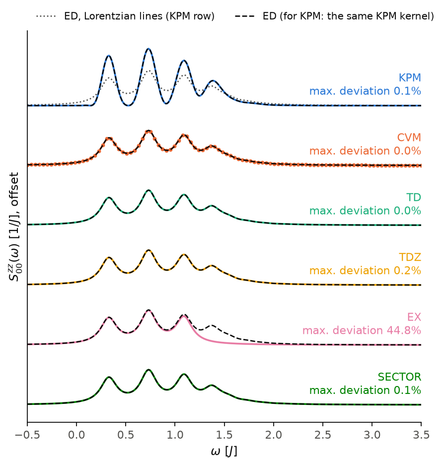
The figure shows the local correlator \(S^{zz}_{00}(\omega)\) at the edge of
a Heisenberg chain with \(n=10\), computed with six methods and the same
\(\delta=0.1\). The dashed lines are ED. The number next to each curve is the
largest deviation from ED, relative to the peak height. CVM, TD, TDZ and
SECTOR fall on the exact Lehmann sum. The KPM lines are narrower and taller
than the Lorentzian lines of ED (dotted). Compared with ED and the same KPM
kernel, KPM agrees to 0.1 per cent. EX with nex=20 misses all the weight
above \(\omega\approx1.2J\), because the states that carry it are not among
its 20 states.
Code of this figure (docs/figures/correlator-methods_comparison/)
# Local spin correlator S^zz_00(omega) of the open spin-1/2 Heisenberg chain
# from every DMRG submode, each against the exact Lehmann sum with the same
# broadening.
import numpy as np
from dmrgpy import spinchain

n = 10
delta = 0.1
es = np.linspace(-0.5, 3.5, 300)
es_cvm = np.linspace(-0.5, 3.5, 100)  # CVM solves one linear system per point

sc = spinchain.Spin_Chain(["S=1/2"]*n)
sc.set_hamiltonian(sum(sc.Sx[i]*sc.Sx[i+1] + sc.Sy[i]*sc.Sy[i+1]
                       + sc.Sz[i]*sc.Sz[i+1] for i in range(n-1)))
sc.maxm, sc.nsweeps, sc.cutoff = 60, 14, 1e-12
sc.kpmmaxm, sc.cvm_maxm = 60, 60
pair = (sc.Sz[0], sc.Sz[0])


def spectrum(**kw):
    return np.asarray(sc.get_dynamical_correlator(name=pair, delta=delta,
                                                  **kw)[1]).real


ed = spectrum(mode="ED", submode="ED", es=es)
ed_cvm = spectrum(mode="ED", submode="ED", es=es_cvm)
ed_kpm = spectrum(mode="ED", submode="KPM", es=es)  # the same kernel as KPM

runs = {"KPM": dict(es=es), "CVM": dict(es=es_cvm),
        "TD": dict(es=es, dt=0.05), "TDZ": dict(es=es, dt=0.05),
        "EX": dict(es=es, nex=20), "SECTOR": dict(es=es, nex=30)}
y = {"y_" + m: spectrum(submode=m, **kw) for m, kw in runs.items()}

np.savez("data.npz", methods=list(runs), es=es, es_cvm=es_cvm, ed=ed,
         ed_cvm=ed_cvm, ed_kpm=ed_kpm, **y)
import numpy as np
import style

d = np.load("data.npz")
methods = [str(m) for m in d["methods"]]
es, es_cvm = d["es"], d["es_cvm"]
offset = 1.05*max(np.max(d["y_" + m]) for m in methods)
# ED reference of each method: KPM against ED with the same kernel
ref = {m: d["ed_cvm"] if m == "CVM" else d["ed_kpm"] if m == "KPM" else d["ed"]
       for m in methods}
residual = {m: np.max(np.abs(d["y_" + m] - ref[m]))/np.max(np.abs(ref[m]))
            for m in methods}


def draw(theme):
    c = style.colors(theme)
    fig, ax = style.figure(1)
    fig.set_size_inches(6.4, 6.4)
    for k, m in enumerate(methods):
        sh = (len(methods) - 1 - k)*offset
        if m == "KPM":
            ax.plot(es, d["ed"] + sh, color=c["ink2"], ls=":",
                    lw=style.LW_REF, label="ED, Lorentzian lines (KPM row)")
            ax.plot(es, d["ed_kpm"] + sh, **style.reference(theme), zorder=3)
        else:
            ax.plot(es, d["ed"] + sh, **style.reference(theme), zorder=3,
                    label="ED (for KPM: the same KPM kernel)" if k == 1 else None)
        ax.plot(es_cvm if m == "CVM" else es, d["y_" + m] + sh,
                color=c["series"][k], lw=style.LW,
                marker="o" if m == "CVM" else None, ms=2.5)
        ax.text(es[-1], sh + 0.12*offset,
                "%s\nmax. deviation %.1f%%" % (m, 100*residual[m]),
                ha="right", va="bottom", color=c["series"][k])
    ax.set_xlim(es[0], es[-1])
    ax.set_xlabel(r"$\omega$ [$J$]")
    ax.set_ylabel(r"$S^{zz}_{00}(\omega)$ [$1/J$], offset")
    ax.set_yticks([])
    ax.legend(loc="lower left", bbox_to_anchor=(0.0, 1.0), ncol=2)
    return fig


style.main(draw, "correlator-methods_comparison")
pair = (sc.Sz[0], sc.Sz[0])
(x, y) = sc.get_dynamical_correlator(submode="CVM", name=pair, es=es, delta=0.1)
(x, y) = sc.get_dynamical_correlator(submode="TD", name=pair, es=es, delta=0.1, dt=0.05)
(x, y) = sc.get_dynamical_correlator(submode="EX", name=pair, es=es, delta=0.1, nex=20)
(x, y) = sc.get_dynamical_correlator(mode="ED", submode="ED", name=pair, es=es, delta=0.1)
Keywords of each method
The accuracy of every method also depends on
the ground state itself, so maxm and nsweeps (Ground state) come first.
sc.kpmmaxm(KPM): the bond dimension of the Chebyshev vectors. Increase it until the spectrum stops changing.sc.kpm_scale(KPM, default 0.7): how much of \([-1,1]\) the spectrum of \(H\) fills after rescaling. Do not go below 0.5; the calculation raises an error when the expansion becomes unstable.sc.kpm_n_scale(KPM, default 1): a positive integer that multiplies the number of Chebyshev moments, for a line sharper than \(2\delta\).sc.kpm_extrapolate = True(KPM): computes the moments for the broadeningkpm_extrapolate_factortimesdelta(default 2, so half as many moments) and extrapolates the sequence to the full count. On a Heisenberg chain of 10 sites the line agrees with the full calculation within 2 per cent of its peak, at half the cost. Check it against the full calculation on a small chain before using it in a scan.kernel=(KPM): how the moments become a spectrum,"jackson"(default),"lorentz","plain"or"hodc". The last is the high-order kernel of arXiv:2512.03149, withhodc_order(default 6) andhodc_eta(defaultdelta). It is more accurate where the spectrum is a smooth continuum, but it can be slightly negative and is more sensitive to a smallkpmmaxm. Seeexamples/dynamical_correlator/hodc_VS_jackson_kernel.sc.kpm_energy_truncate=True(KPM,itensor_version=3and"python"): energy truncation of Holzner et al., PRB 83, 195115 (2011). It allowskpm_scalewell below 0.5, so that more moments are spent on the low-energy window. It is slower per moment. The settings arekpm_truncate_dK(increase until converged, 30 is a good value),kpm_truncate_nsweepsandkpm_truncate_threshold. Seeexamples/dynamical_correlator/dynamical_correlator_kpm_energy_truncation.sc.cvm_maxmandsc.cvm_tol(CVM): the bond dimension of the correction vector and the relative tolerance of its solver (default \(10^{-5}\)). If a frequency point warns that it did not converge, increasecvm_maxm.sc.cvm_solver="variational"(CVM,itensor_version=3and"python", only forAequal toB^dagger): the dynamical DMRG of Jeckelmann, PRB 66, 045114 (2002). The correction vector is found by minimizing a functional with two-site sweeps, so the truncation is part of the ansatz. Setcvm_nsweepsandcvm_maxm. The default"cg"works on every backend.sc.inverse_solver(CVM_explicit): the solver of each resolvent, for any pairA,B. By default two-site sweeps on"python", since the resolvent is not Hermitian, and BiCGSTAB on the other backends (see Operators).Nandnkry(ROOTN, defaults 8 and 20): the number of steps and the Krylov dimension. LargerNhelps at high frequency whennkryis small.dtanddamping_periods(TD and TDZ): the time step, and the total time \(T\) in units of \(1/\delta\) (default 6). The resolution is set by \(T\).dampingandpredict(TD): the time window,"exp"(default, a Lorentzian line),"gaussian"(faster decaying tails, line 1.2 times wider) or"parzen", and linear prediction of \(C(t)\) to longer times (defaultTrue), which makes the line sharper and more accurate when the simulated time is short.alpha0andn_max(TDZ, defaults 0.1 and 4): the angle of the time contour and the order of the expansion back to real time. A largeralpha0needs a smaller bond dimension but a largern_max, at most 4.nex(EX and SECTOR): the number of states in the sum. Withreturn_poles=True, SECTOR also returns the poles and their weights, andinfo["captured"]is the fraction of the weight \(\langle\mathrm{GS}|B^\dagger B|\mathrm{GS}\rangle\) they account for. A warning appears below 0.9; increasenexthen.nkry(TASK, default 100): the number of Lanczos steps, about the number of poles. Withreturn_poles=True, TASK returns(es, y, info):info["omega"]andinfo["weight"]are the poles and their weights,info["elastic"]the weight \(\langle A\rangle\langle B\rangle\) at \(\omega=0\), andinfo["variance"]the two-site variance of each pole, \(\lVert P^{2\perp}H|\alpha\rangle\rVert^2\). Its square root is an error bar on the energy of the pole; increasemaxmuntil it is small for the poles you need.info["missing_weight"]is the sum rule \(\langle A B\rangle\) minus all the weights. It is not zero when \(B\) changes more than one site of the ground state: a bond operator, or \(c_i\) on a state of mixed fermion parity, such as a degenerate pair of Majorana ground states. The variance does not see this loss. A warning appears when it is above \(10^{-6}\) of the weight; increasemaxmthen.
Reusing the KPM moments
The Chebyshev moments are the expensive part of KPM. We can compute them once and build the spectrum with several kernels:
from dmrgpy import kpmdmrg
mus, emin, emax, scale, npol, delta = sc.get_dynamical_correlator_moments(
        name=(sc.Sz[0], sc.Sz[0]), delta=0.1)
(x, y) = kpmdmrg.dynamical_correlator_from_moments(mus, emin, emax, scale,
        npol, es, kernel="hodc", delta=delta)
Degenerate ground states
With mode="ED", submode="ED", a degenerate ground state is handled by
averaging the correlator over all the states with excitation energy below
dex (default \(10^{-5}\)), with equal weights. This is a hard cutoff, so in
a scan where a level splitting crosses dex (a Zeeman field, for example)
the result jumps. A warning appears when a level is close to dex. For a
scan, use a small temperature instead, T=0.01, which weights the states
with Boltzmann factors and changes smoothly (Finite temperature). See
examples/kondo/atom_iets_orbital_resolved.
Non-Hermitian Hamiltonians
For a non-Hermitian \(H\) (Excited states) the ground state is a pair of left and
right eigenstates, and the correlator is
\(\langle\psi_L|A(z)B|\psi_R\rangle\). submode="KPM" then uses the
non-Hermitian KPM of PRL 130, 100401,
and needs E_max, an upper bound on the spectral radius of \(H\). It
recomputes the moments at every frequency, so it is much slower. "CVM",
"CVM_explicit" and "EX" also work; the other submodes raise an error.
Non-Hermitian KPM works with mode="ED", itensor_version=3,
"python" and "julia_live". See examples/non_hermitian/nhkpm_v3_VS_ED.